Japanese Dependency Structure Analysis Based on Support Vector Machines

(1)

Japanese D e p e n d e n c y Structure Analysis

Based on Support Vector Machines

T a k u K u d o and Y u j i M a t s u m o t o G r a d u a t e School of I n f o r m a t i o n Science, N a r a I n s t i t u t e of Science a n d Technology

{taku-ku, matsu}@is, aist-nara, ac. jp

. . . . . - " r

A b s t r a c t

This paper presents a method of Japanese dependency structure analysis based on Sup-- port Vector Machines (SVMs). Conventional parsing techniques based on Machine Learn- ing framework, such as Decision Trees and Maximum Entropy Models, have difficulty in selecting useful features as well as find- ing appropriate combination of selected features. On the other hand, it is well-known that SVMs achieve high generalization performance even with input data of very high dimensional feature space. Furthermore, by introducing the Kernel principle, SVMs can carry out the training in high-dimensional • spaces with a smaller computational cost independent of their dimensionality. We apply SVMs to Japanese dependency structure iden- tification problem. Experimental results on Kyoto University corpus show that our system achieves the accuracy of 89.09% even with small training data (7958 sentences).

1 I n t r o d u c t i o n

Dependency structure analysis has been rec- ognized as a basic technique in Japanese sentence analysis, and a number of stud- ies have been proposed for years. Japanese dependency structure is usually defined in terms of the relationship between phrasal units called 'bunsetsu' segments (hereafter "chunks~). Generally, dependency structure analysis consists of two steps. In the first step, dependency matrix is constructed, in which each element corresponds to a pair of chunks and represents the probability of a dependency relation between them. The second step is to find the optimal combination of dependencies to form the entire sentence.

In previous approaches, these probabilites of dependencies axe given by manually constructed rules. However, rule-based approaches have problems in coverage and con-

sistency, since there are a number of features that affect the accuracy of the final results, and these features usually relate to one another.

On the other hand, as large-scale tagged corpora have become available these days, a number of statistical parsing techniques which estimate the dependency probabilities using such tagged corpora have been devel- oped(Collins, 1996; Fujio and Matsumoto, 1998). These approaches have overcome the systems based on the rule-based approaches. Decision Trees(Haruno et al., 1998) and Max- imum Entropy models(Ratnaparkhi, 1997; Uchimoto et al., 1999; Charniak, 2000) have been applied to dependency or syntactic structure analysis. However, these models require an appropriate feature selection in order to achieve a high performance. In addition, ac- quisition of an efficient combination of features is difficult in these models.

In recent years, new statistical learning techniques such as Support Vector Machines (SVMs) (Cortes and Vapnik, 1995; Vap- nik, 1998) and Boosting(Freund and Schapire, 1996) are proposed. These techniques take a strategy that maximize the margin between critical examples and the separating hyperplane. In particular, compared with other conventional statistical learning algorithms, SVMs achieve high generalization even with training data of a very high dimension. Fur- thermore, by optimizing the Kernel function, SVMs can handle non-linear feature spaces, and carry out the training with considering combinations of more than one feature.

Thanks to such predominant nature, SVMs deliver state-of-the-art performance in real- world applications such as recognition of hand-written letters, or of three dimensional images. In the field of natural language processing, SVMs are also applied to text categorization, and are reported to have achieved

(2)

high accuracy without falling into over-fitting even with a large number of words taken as the features (Joachims, 1998; Taira and Haruno, 1999).

In this paper, we propose an application of SVMs to Japanese dependency structure analysis. We use the features that have been studied in conventional statistical dependency analysis with a little modification on them.

2 S u p p o r t V e c t o r M a c h i n e s

2.1 O p t i m a l H y p e r p l a n e

Let us define the training d a t a which belong either to positive or negative class as follows.

(xl, vl),..., (xi, v~),..., (x~, v~)

x i E a n , y / E { + i , - 1 }

xi is a feature vector of i-th sample, which is represented by an n dimensional vector (xi = ( f l , . . . , f f , ) E Rn). Yi is a scalar value that specifies the class (positive(+l) or negative(- l) class) of i-th data. Formally, we can define the p a t t e r n recognition problem as a learning and building process of the decision function

f: lq. n ~ {=i::l}.

In basic SVMs framework, we try to sepa- r a t e the positive and negative examples in the training data by a linear hyperplane written a s :

( w - x ) + b = 0 w e R n , b e R . (1)

It is supposed that the farther the positive and negative examples are separated by the discrimination function, the more accurately we could separate unseen test examples with high generalization performance. Let us consider two hyperplanes called separating hyperplanes:

( w - x i ) + b _ > 1 i f ( y i = l ) (2) ( w - x i ) + b _< - 1 if (Yi = - - 1 ) . (3)

(2) (3) can be written in one formula as:

w[(w- x~) + b] >_ 1

(i = 1 , . . . , 0 .

(4)

Distance from the separating hyperplane to the point xi can be written as:

d(w, b; xi) = Iw" ~ + bl

Ilwll

Thus, the margin between two separating hyperplanes can be written as:

rain d ( w , b ; x i ) + rain d ( w , b ; x i )

x i ;Yi = l x i ; y i = - - i

= rain I w ' x i + b I + rain

x,;y,=l

Ilwll

x,;~,=-i

2

Ilwll"

Iw" xi + bl

IIwll

To maximize this margin, we should minimize Hwll. In other words, this problem becomes equivalent to solving the following optimization problem:

Minimize: L(w) = ½l[wl[ 2 Subject t o : y i [ ( w - x i ) + b ] > 1 ( i = l , . . . , l ) .

Furthermore, this optimization problem can be rewritten into t h e dual form problem: Find the Lagrange multipliers c~i >_ O(i = 1 , . . . , l) so that:

Maximize:

l 1 l

-

~ a~c~y~y~(xi,

xj) (5)

L(~) = Z ~

_~

i = l ",j:'= 1

Subject to:

l

~ _> 0, ~ ~y~ = 0 (i = 1 , . . . , l)

i = 1

In this dual form problem, xi with non-zero ai is called a Support Vector. For the Support Vectors, w and b can thus be expressed as follows

w = E o~iYi x i b = w • x i - Yi.

i ; x i 6 S V s

T h e elements of t h e set S V s are the Support Vectors that lie on the separating hyperplanes. Finally, the decision function ff : R n ---r {::El} can be written as:

f ( x ) = s g n ( i ; x , ~esvs c~iYi (xi - x) + b)(6)

= sgn ( w - x + b).

2.2 S o f t M a r g i n

In the case where we cannot separate training examples linearly, "Soft Margin" m e t h o d forgives some classification errors t h a t may be caused by some noise in the training examples. First, we introduce non-negative slack vari- ables, and (2),(3) are rewritten as:

(3)

In this case, we minimize t h e following value instead of 1 _llwll2

l

-Ilwll + c (7)

i----1

The first t e r m in (7) specifies t h e size of margin and the second t e r m evaluates how far the training d a t a are away from the optimal separating hyperplane. C is t h e p a r a m e t e r that defines the balance of two quantities. If we make C larger, the more classification errors are neglected.

Though we omit t h e details here, minimiza- tion of (7) is reduced to t h e problem to minimize the objective function (5) under the following constraints.

0 < ai _< c , a y/= 0 (i = 1 , . . . , z)

Usually, the value of C is estimated experi- mentally.

2.3 K e r n e l F u n c t i o n

In general classification problems, there are cases in which it is unable to separate the training d a t a linearly. In such cases, the training data could be separated linearly by ex- panding all combinations of features as new ones, and projecting t h e m onto a higher- dimensional space. However, such a naive approach requires enormous computational overhead.

Let us consider t h e case where we project the training data x onto a higher-dimensional space by using projection function • 1 As we pay attention to the objective function (5) and the decision function (6), these functions depend only on t h e dot products of t h e in- p u t training vectors. If we could calculate the dot products from xz and x2 directly without considering the vectors ~(xz) a n d ¢(x2) pro- jected onto the higher-dimensional space, we can reduce the computational complexity considerably. Namely, we can reduce the computational overhead if we could find t h e function K that satisfies:

~ ( x l ) " ¢(x2) ---- K(Xl~ x2). (8)

On the other hand, since we do not need itself for actual learning a n d classification,

1In general, ,It(x) is a m a p p i n g i n t o H i l b e r t space.

all we have to do is to prove the existence of that satisfies (8) provided the function K is selected properly. It is known t h a t (8) holds if and only if the function K satisfies the Mercer condition (Vapnik, 1998).

In this way, instead of projecting the training data onto t h e high-dimensional space, we can decrease t h e c o m p u t a t i o n a l overhead by replacing the dot products, which is calculated in optimization a n d classification steps, with the function K .

Such a function K is called a K e r n e l f u n c - t i o n . Among t h e m a n y kinds of Kernel functions available, we will focus on t h e d-th polynomial kernel:

K ( x l , x 2 ) = (Xl'X2--t-1) a. (9)

Use of d-th polynomial kernel function allows us to build an optimal separating hyperplane which takes into account all combination of features up to d.

Using a Kernel function, we can rewrite the decision function as:

y = sgn (i;x~ ~esVs

oLiyiK(xi,x)+b).

(10)

3 D e p e n d e n c y A n a l y s i s u s i n g S V M s

3.1 T h e P r o b a b i l i t y M o d e l

This section describes a general formulation of the probability model and parsing techniques for Japanese statistical dependency analysis.

First of all, we let a sequence of chunks be

{bz,b2...,bm}

by B, and the sequence d e p e n d e n c y p a t t e r n be

{Dep(1),Dep(2),...,Dep(m -

1)} by D, where

Dep(i) = j

means t h a t t h e chunk b~ depends on (modifies) t h e chunk bj.

In this framework, we suppose t h a t the dependency sequence D satisfies the following constraints.

1. Except for t h e rightmost one, each chunk depends on (modifies) exactly one of the chunks appearing to the right.

2. Dependencies do not cross each other.

Statistical d e p e n d e n c y structure analysis is defined as a searching problem for the dependency p a t t e r n D t h a t maximizes the conditional probability

P(DIB )

of the in-

(4)

put sequence under the above-mentioned constraints.

Dbest =

argmax

P(D[B)

D

If we assume that the dependency probabilities are mutually independent,

P ( D I B )

could be rewritten as:

r n - 1

P ( D I B ) = ~I P ( D e p ( i ) = j

Ifit) i = 1

fit = { f l , . . . , f n } e R n.

P(Dep(i) =

J If0) represents the probability that

bi

depends on (modifies) b t. fit is an n dimensional feature vector that represents var- ious kinds of linguistic features related with the chunks

bi

and

b t.

We obtain

Dbest

taking into all the combination of these probabilities. Generally, the optimal solution

Dbest

C a n be identified by using

bottom-up algorithm such as CYK algorithm. Sekine suggests an efficient parsing technique for Japanese sentences that parses from the end of a sentence(Sekine et al., 2000). We apply Sekine's technique in our experiments. ..?

3.2 T r a i n i n g w i t h S V M s

In order to use SVMs for dependency analysis, we need to prepare positive and negative examples since SVMs is a binary classifier. We adopt a simple and effective method for our purpose: Out of all combination of two chunks in the training data, we take a pair of chunks that axe in a dependency relation as a positive example, and two chunks that appear in a sentence but are not in a dependency relation as a negative example.

LJ (f J,y t) = {(f12,y12), (f23,v23),

~l_<j<m

---, (fro-1 m, Ym-1 m)}

fij = { f l , - - - , f n ) e R n

Yij E

(Depend(q-l), N o t - D e p e n d ( - 1 ) }

Then, we define the dependency probability

P ( Dep( i) = j l f'ij ):

P(Dep(i)

= j

I f'ij) =

(11)

(11) shows that the distance between test data fr O and the separating hyperplane is put into the sigmoid function, assuming it represents the probability value of the dependency relation.

We adopt this method in our experiment to transform the distance measure obtained in SVMs into a probability function and an- alyze dependency structure with a fframework of conventional probability model 2

3.3 S t a t i c a n d D y n a m i c F e a t u r e s

Features that are supposed to be effective in Japanese dependency analysis are: head words and their parts-of-speech, particles and inflection forms of the words that appear at the end of chunks, distance between two chunks, existence of punctuation marks. As those are solely defined by the pair of chunks, we refer to them as s t a t i c f e a t u r e s .

Japanese dependency relations are heavily constrained by such static features since the inflection forms and postpositional particles constrain the dependency relation. However, when a sentence is long and there are more than one possible dependents, static features, by themselves cannot determine the correct dependency. Let us look at the following example.

watashi-ha kono-hon-wo motteim josei-wo sagasiteiru I-top, this book-acc, have, lady-acc, be looking for

In this example, "kono-hon-wo(this book- acc)" may modify either of "motteiru(have)" or "sagasiteiru(be looking for)" and cannot be determined only with the static features. However, "josei-wo (lady-acc)" can modify the only the verb "sagasiteiru,". Knowing such information is quite useful for resolv- ing syntactic ambiguity, since two accusative noun phrses hardly modify the same verb. It is possible to use such information if we add new features related to other modifiers. In the above case, the chunk "sagasiteiru" can receive a new feature of accusative modification (by "josei-wo") during the parsing process, which precludes the chunk "kono-hon- wo" from modifying "sagasiteiru" since there is a strict constraint about double-accusative

(5)

modification that will be learned from training examples. We decided to take into consideration all such modification information by using functional words or inflection forms of modifiers.

Using such information about modifiers in the training phase has no difficulty since they are clearly available in a tree-bank. O n the other hand, they are not known in t h e parsing phase of the test data. This problem can be easily solved if we adopt a b o t t o m - u p parsing algorithm and attach the modification information dynamically to the newly constructed phrases (the chlmks t h a t become t h e head of the phrases). As we describe later we apply a beam search for parsing, a n d it is possible to keep several intermediate solutions while sup- pressing the combinatorial explosion.

We refer to the features t h a t are a d d e d in- crementally during the parsing process as d y - n a m i c f e a t u r e s .

4 E x p e r i m e n t s a n d D i s c u s s i o n

4.1 E x p e r i m e n t s S e t t i n g

We use Kyoto University text corpus (Ver- sion 2.0) consisting of articles of Mainichi newspaper annotated with dependency structure(Kurohashi and Nagao, 1997). 7,958 sentences from the articles on J a n u a r y 1st to Jan- uary 7th are used for the training data, and 1,246 sentences from the articles on January 9th are used for the test data. For t h e kernel function, we used the polynomial function (9). We set the soft margin parameter C to be 1.

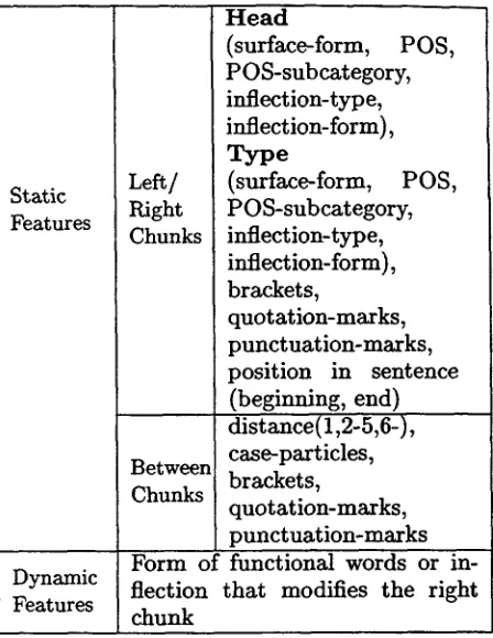
The feature set used in t h e experiments are shown in Table 1. The static features are ba- sically taken from Uchimoto's list(Uchimoto et al., 1999) with little modification. I n Table 1, 'Head' means the rightmost content word in a chunk whose part-of-speech is n o t a functional category. 'Type' means the rightmost functional word or the inflectional form of the rightmost predicate if there is no functional word in the chunk. T h e static features in- clude the information on existence of brackets, question marks and p u n c t u a t i o n marks etc. Besides, there are features t h a t show the relative relation of two chunks, such as distance, and existence of brackets, quotation marks and p u n c t u a t i o n marks between them. For dynamic features, we selected functional words or inflection forms of t h e rightmost predicates in the chunks that a p p e a r between two chunks and d e p e n d on t h e modi- flee. Considering data sparseness problem, we

Static Features

Dynamic Features

H e a d

(surface-form, POS, POS-subcategory, inflection-type, inflection-form), T y p e

Left/ (surface-form, POS, Right POS-subcategory, Chunks inflection-type,

inflection-form), brackets,

quotation-marks, punctuation-marks, position in sentence

(beginning, end) distance(I,2-5,6-), Between case-particles, Chunks brackets,

quotation-marks, punctuation-marks Form of functional words or inflection that modifies the right chunk

Table 1: Features used in experiments

apply a simple filtering based on the part-of- speech of functional words: We use the lexical form if the word's P O S is particle, adverb, ad- nominal or conjunction. We use t h e inflection form if the word has inflection. We use the P O S tags for others.

4.2 R e s u l t s o f E x p e r i m e n t s

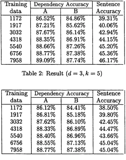
Table 2 shows t h e result of parsing accuracy under the condition k = 5 (beam width), and d = 3 (dimension of t h e polynomial functions used for the kernel function).

This table shows two types of dependency accuracy, A a n d B. T h e training d a t a size is measured by the n u m b e r of sentences. T h e accuracy A means the accuracy of t h e entire dependency relations. Since Japanese is a head- final language, t h e second chunk from the end of a sentence always modifies t h e last chunk. T h e accuracy B is calculated by excluding this dependency relation. Hereafter, we use t h e accuracy A, if it is not explicitly specified, since this measure is usually used in other litera- ture.

4.3 E f f e c t s o f D y n a m i c F e a t u r e s

Table3 shows t h e accuracy when only static features are used. Generally, the results with

[image:5.596.347.571.66.356.2]

(6)

Training data 1172 1917 3032 4318 5540 6756 7958

Dependency Accuracy

86.52%

87.21%

87.67%

88.35%

88.66%

88.77%

89.09%

B

84.86% 85.62% 86.14% 86.91% 87.26% 87.38% 87.74%

Sentence Accuracy

39.31%

40.06%

42.94%

44.15%

45.20%

45.36%

46.17%

Table 2: Result (d = 3, k = 5)

Training data 1172 1917 3032 4318 5540 6756 7958

Dependency Accuracy

A

86.12%

86.81%

87.62%

88.33%

88.40%

88.55%

88.77%

B 84.41% 85.18% 86.10% 86.89% 86.96% 87.13% 87.38%

Sentence Accuracy

38.50%

39.80%

42.45%

44.47%

43.66%

45.04%

Table 3: Result without dynamic features (d = 3, k = 5)

dynamic feature set is better than the results without them. The results with dynamic features constantly outperform that with static features only. In most of cases, the improvements is significant. In the experiments, we restrict the features only from the chunks that appear between two chunks being in consideration, however, dynamic features could be also taken from the chunks that appear not between the two chunks. For example, we could also take into consideration the chunk that is modified by the right chunk, or the chunks

W

m.5

8,r

/

~ 0 ~o0 4c00 $000 ~ 0 0 7Oo0 Nt~Iber of TriL~img 0,11~a (l~'sl~c~)

Figure 1: Training Data vs Accuracy

Dimension Dependency Sentence of Kernel Accuracy Accuracy

1 2 3 4

N / A 86.87%

87.67%

8'7.72%

N / A 40.60%

4 2 . 9 4 %

42.78%

Table 4: Dimension vs. Accuracy (3032 sentences, k = 5)

that modify the left chunk. We leave experiment in such a setting for the future work.

4 . 4 T r a i n i n g d a t a vs. A c c u r a c y

Figure 1 shows the relationship between the size of the training data and the parsing accuracy. This figure shows the accuracy of with and without the dynamic features.

The parser achieves 86.52% accuracy for test data even with small training data (1172 sentences). This is due to a good character- istic of SVMs to cope with the data sparseness problem. Furthermore, it achieves almost 100% accuracy for the training data, showing t h a t the training data are completely separated by appropriate combination of features. Generally, selecting those specific features of the training data tends to cause overfitting, and accuracy for test data may fall. However, the SVMs method achieve a high accuracy not only on the training data but also on the test data. We claim that this is due to the high generalization ability of SVMs. In addition, observing at the learning curve, further im- provement will be possible if we increase the size of the training data.

[image:6.596.87.308.67.348.2]

4.5 K e r n e l F u n c t i o n vs. A c c u r a c y

Table 4 shows the relationship between the dimension of the kernel function and the parsing accuracy under the condition k -- 5.

As a result, the case of d ---- 4 gives the best accuracy. We could not carry out the training in realistic time for the case of d = 1.

[image:6.596.334.528.67.143.2] [image:6.596.93.301.568.715.2]

(7)

Beam Dependency Sentence W i d t h Accuracy Accuracy

1 3 5 7 10 15

88.66% 88.74% 8 8 . 7 7 %

88.76% 88.67% 88.65%

45.76% 45.20% 4 5 . 3 6 % 4 5 . 3 6 % 45.28% 45.28%

Table 5: Beam width vs. Accuracy (6756 sentences, d = 3)

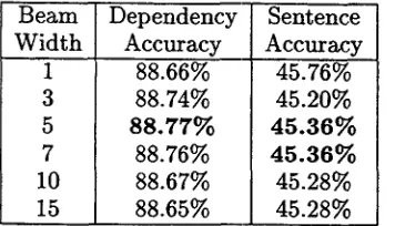
4.6 B e a m w i d t h vs. A c c u r a c y

Sekine (Sekine et al., 2000) gives an interest- ing report about the relationship between the beam width and t h e parsing accuracy. Gener- ally, high parsing accuracy is expected when a large b e a m width is employed in the dependency structure analysis. However, the result is against our intuition. T h e y report that a beam width between 3 and 10 gives t h e best parsing accuracy, and parsing accuracy falls down with a width larger t h a n 10. This result suggests t h a t Japanese dependency structures may consist of a series of local optimization processes.

We evaluate the relationship between the beam w i d t h and the parsing accuracy. Table 5 shows their relationships under t h e condition d = 3, along with the changes of the b e a m width from k = 1 to 15. T h e best parsing accuracy is achieved at k ---- 5 and the best sentence accuracy is achieved at k = 5 and

k = 7 .

We have to consider how we should set the beam width that gives t h e best parsing accuracy. We believe that t h e b e a m width t h a t gives the best parsing accuracy is related not only with the length of t h e sentence, b u t also with the lexical entries and parts-of-speech that comprise the chunks.

4.7 C o m m i t t e e b a s e d a p p r o a c h

Instead of learning a single c l a s s i e r using all training data, we can make n classifiers di- viding all training data by n, a n d t h e final result is decided by their voting. This approach would reduce computational overhead. T h e use of multi-processing computer would help to reduce their training time considerably since all individual training can be carried out in parallel.

To investigate the effectiveness of this method, we perform a simple experiment: Di-

viding all training data (7958 sentences) by 4, the final dependency score is given by a weighted average of each scores. This simple voting approach is shown to achieve the accuracy of 88.66%, which is nearly the same accuracy achieved 5540 training sentences.

In this experiment, we simply give an equal weight to each classifier. However, if we op- timized the voting weight more carefully, the further improvements would be achieved (Inui and Inni, 2000).

4.8 C o m p a r i s o n w i t h R e l a t e d Work

Uchimoto (Uchimoto et al., 1999) and Sekine (Sekine et al., 2000) report t h a t using Kyoto University Corpus for their training and test- ing, they achieve around 87.2% accuracy by building statistical model based on M a x i m u m Entropy framework. For t h e training data, we used exactly t h e same d a t a t h a t they used in order to make a fair comparison. In our experiments, the accuracy of 89.09% is achieved using same training data. Our model outperforms Uchimoto's model as far as the accura- cies are compared.

Although Uchimoto suggests t h a t the im- portance of considering combination of features, in ME framework we must expand these combination by introducing new feature set. Uchimoto heuristically selects "effective" combination of features. However, such a manual selection does not always cover all relevant combinations that are i m p o r t a n t in the determination of dependency relation.

We believe t h a t our model is better t h a n others from the viewpoints of coverage and consistency, since our model learns the combination of features without increasing the computational complexity. If we want to recon- sider them, all we have to do is j u s t to change the Kernel function. The computational complexity depends on the n u m b e r of s u p p o r t vectors not on the dimension of t h e Kernel function.

4.9 F u t u r e W o r k

T h e simplest and most effective way to achieve better accuracy is to increase t h e training data. However, the proposed m e t h o d that uses all candidates t h a t form dependency relation requires a great a m o u n t of time to com- p u t e the separating h y p e r p l a n e a s t h e size of the training d a t a increases. T h e experiments given in this p a p e r have actually taken long

[image:7.596.137.315.64.166.2]

(8)

training time 3

To handle large size of training data, we have to select only the related portion of examples that are effective for the analysis. This will reduce the training overhead as well as the analysis time. The committee-based approach discussed section 4.7 is one method of coping with this problem. For future research, to reduce the computational overhead, we will work on methods for sample selection as follows:

• Introduction of constraints on non- dependency

Some pairs of chunks need not consider since there is no possibility of dependency between them from grammatical constraints. Such pairs of chunks are not necessary to use as negative examples in the training phase. For example, a chunk within quotation marks may not modify a chunk that locates outside of the quotation marks. Of course, we have to be careful in introducing such constraints, and they should be learned from existing corpus.

• Integration with other simple models Suppose that a computationally light and moderately accuracy learning model is obtainable (there are actually such systems based on probabilistic parsing models). We can use the system to output some redundant parsing results and use only those results for the positive and negative examples. This is another way to reduce the size of training data.

• Error-driven data selection

We can start with a small size of training data with a small size of feature set. Then, by analyzing held-out training data and selecting the features that affect the parsing accuracy. This kind of grad- ual increase of training data and feature set will be another method for reducing the computational overhead.

5 S u m m a r y

This paper proposes Japanese dependency analysis based on Support Vector Machines. Through the experiments with Japanese bracketed corpus, the proposed method achieves a high accuracy even with a small

3With AlphaServer 8400 (617Mhz), it took 15 days to train with 7958 sentences.

training data and outperforms existing methods based on Maximum Entropy Models. The result shows t h a t Japanese dependency analysis can be effectively performed by use of SVMs due to its good generalization and non- overfitting characteristics.

R e f e r e n c e s

Eugene Charniak. 2000. A maximum-entropy- inspired parser. In Processing of the NAACL

2000, pages 132-139.

Michael Collins. 1996. A new statistical parser based on bigram lexical dependencies. In Pro-

ceedings of the ACL '96, pages 184-191.

C. Cortes and Vladimir N. Vapnik. 1995. Support Vector Networks. Machine Learning, 20:273- 297.

Y. Freund and Schapire. 1996. Experiments with a new Boosting algoritm. In 13th International

Conference on Machine Learning.

Masakazu Fujio and Yuji Matsumoto. 1998. Japanese Dependency Structure Analysis based on Lexicalized Statistics. In Proceedings of

EMNLP '98, pages 87-96.

Msahiko Haruno, Satoshi Shirai, and Yoshifumi Ooyama. 1998. Using Decision Trees to Con- struct a Partial Parser. In Proceedings of the

COLING '98, pages 505-511.

Takashi Inui and Kentaro Inui. 2000. Committe- based Decision Making in Probabilistic Partial Parsing. In Proceedings of the COLING 2000,

pages 348-354.

Thorsten Joachims. 1998. Text Categorization with Support Vector Machines: Learning with Many Relevant Features. In European Confer-

ence on Machine Learning (ECML).

Sadao Kurohashi and Makoto Nagao. 1997. Kyoto University text corpus project. In Proceedings

of the ANLP, Japan, pages 115-118.

John C. Platt. 1999. Probabilistic Outputs for Support Vector Machines and Comparisons to Regularized Likelihood Methods. In Advances

in Large Margin Classifiers. MIT Press.

Adwait Ratnaparkhi. 1997. A Liner Observed Time Statistical Parser Based on Maximum En- tropy Models. In Proceedings of EMNLP 'gZ

Satoshi Sekine, Kiyotaka Uchimoto, and Hitoshi Isahara. 2000. Backward Beam Search Algo- rithm for Dependency Analysis of Japanese. In

Proceedings of the COLING 2000, pages 754-

760.

Hirotoshi Taira and Masahiko Haruno. 1999. Fea- ture Selection in SVM Text Categorization. In

AAAI-99.

Kiyotaka Uchimoto, Satoshi Sekine, and Hitoshi Isahara. 1999. Japanese Dependency Structure Analysis Based on Maximum Entropy Models.

In Proceedings of the EA CL, pages 196-203.

Vladimir N. Vapnik. 1998. Statistical Learning