Modeling & Simulation of Supersonic Flow Using McCormack’s Technique

Modeling & Simulation of Supersonic Flow Using

McCormack’s Technique

M. Saif Ullah Khalid*, Afzaal M. Malik**

Abstract—In this work, two-dimensional inviscid supersonic flow around a wedge has been investigated using CFD scheme. The employed scheme is McCormack’s predictor-corrector scheme. Our own code, CFMOD was written using MATLAB environment. Proper boundary conditions and the grid parameters were decided on the basis of standard techniques. The results are verified using classic theories for supersonic flows and a standard CFD package; Fluent. The proper grid generation around the airfoil was decided on the basis of numerical experimentation. Various flow parameters were found to be in good agreement with the results obtained from theory and Fluent.

Index Terms—CFD, Supersonic flow, McCormack’s Scheme, Inverse solution for Prandtl-Mayer function

I. INTRODUCTION

Computational Fluid Dynamics has been converted into a specialized field to find out the solution for many real complex physical problems. Especially, the problems involving the shock waves are of great importance. Now-a-days, many space- marching and time-marching schemes are in use. Some of these schemes capture the effects of shock waves themselves and for others; one has to follow shock-fitting approach in the CFD schemes. The analytical and numerical calculation of supersonic flow parameters around the wedge and sharp-edged airfoils has been the topic of wide research, in the fields of Mechanical engineering, Aerospace engineering and Mathematics. In [1], the authors studied local existence and the uniqueness of weak shock solution in steady supersonic flow past a wedge. The authors [2] constructed an analytical solution for the generation of shock wave as a result of supersonic flow around a wedge. In this work, McCormack’s explicit predictor-corrector scheme has been employed to find out the parameters of the flow-field around the wedge.

Department of Mechanical Engineering College of Electrical & Mechanical Engineering

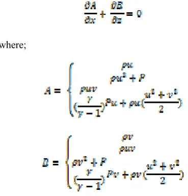
To employ, this numerical procedure, inviscid supersonic flow may be described using following Euler equations. With no source involved,

where;

This partial differential equation is to be solved numerically in the transformed space i.e. computational

ξη-plane.

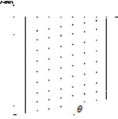
Physically, the flow field may be imagined as shown in Figure 1.

For simplicity, the grid for physical space is shown to be;

Fig. 2: Grid in Physical space

We can use following relations to transform the xy coordinate system into generalized ξη- coordinate system [3].

where;

= Wedge surface =

= Local height of the physical system

where,

= maximum height of the physical system

Now, the computational space will look like a rectangular grid as shown in Figure 3.

Fig. 3: Grid in Computational space

II. GRID GENERATION

As described in [3], to calculate the step size for the downstream space marching, CFL (Courant-Freidrichs-Lewy) criterion may be used.

where, = Mach angle

= flow deflection angle

III. INITIAL & UPPER BOUNDARY CONDITIONS

Initial data line is selected to be at while upper boundary line is . Along these vertical and horizontal lines, at each grid point, the initial data, equal to the uniform upstream flow conditions for Mach, M = 1.8.

IV. NUMERICAL MODELING

To use McCormack’s scheme [3, 4], following relations need to be evaluated.

These relations can be used to represent Euler equations in the computational space, i.e. in the form of generalized coordinates.

This is the required partial differential equation, to be solved numerically using McCormack’s scheme.

V. WALL BOUNDARY CONDITIONS

Only condition that can be imposed as the wall boundary condition is the flow to be tangent to the wall. As described in [3], Abbett’s work can be used to implement the wall boundary conditions. Using this condition, the parameters on the wall can be calculated according to the following scheme.

2). The velocities, calculated from the usual approach may not be tangent to the wall, as shown in the Fig. 4.

Fig. 4: Rotation of flow to fulfill tangency condition

3). The direction of this calculated flow velocity may be calculated using the Prandtl-Mayer function [5, 6].

4). The actual direction of the velocity may be incorporated using following relation.  

It means that the actually flow may be tangent to the wall of the wedge, if the numerically calculated flow be rotated to an angle of .

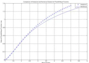
5). Actual Mach number M, with tangent flow to the wall, can be calculated from the following approximation that has been estimated using MATLAB curve fitting tool [7]. It actually represents the inverse solution for the Prandtl-Mayer function.

Fig. 5: Comparison of Numerical & Analytical Results (for air)

6). From these actual values of Mach number, pressure, density and temperature may be calculated [1].

VI.DISCUSSION & COMPARISON OF RESULTS

The results obtained from the numerical solution without involvement of numerical dissipation are discontinuous. If the x and y coordinates of the grid points with unstable numerical results are used, it is obviously noted that this discontinuity arises, right after the production of shock wave at the corner of the wedge. So, to remove this discontinuity, numerical dissipation has been employed. The relation used for this purpose is, as proposed in [3].

For predictor step, numerical dissipation is;

For corrector step, this expression may be used to calculate the numerical dissipation factor, using values of the pressure vector P and A-vector, as estimated in the predictor step.

Fig. 6: Plot of Courant number against Mach for different values of step size

In this figure, represents the grid spacing in the physical plane along vertical direction. From the classic theory of supersonic flow, the calculated results for flow parameters, behind the shock wave are shown in the following table.

Table 1: Theoretical Values for flow parameters behind shock wave

Flow Parameter Value Pressure 131661.705

Temperature 321.81 K

Mach Number 1.623

Density 1.23

As shown in Table 1, the value of Mach number is 1.623, so according to the Fig. 6, the appropriate value of the Courant number is 0.1.

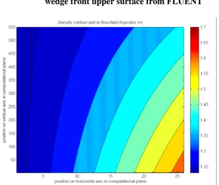
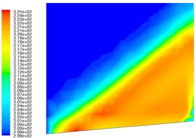
Contour plots for Pressure, Temperature, Density and Mach number, obtained from CFMOD and FLUENT [8] for front upper surface of the wedge foil are shown in Figures 7-14. These plots show that results obtained from CFMOD are in good agreement with those from FLUENT [8] and classic theories of supersonic flow.

Fig. 7: Mach number Contour plot along wedge front upper surface from CFMOD

Figure 8: Mach number Contour plot along wedge front upper surface from FLUENT

Fig. 10: Density Contour plot along wedge front upper surface from FLUENT

Figure 11: Pressure Contour plot along wedge front upper surface using CFMOD

Fig. 12: Pressure Contour plot along wedge front upper surface using FLUENT

Fig. 13: Temperature Contour plot along wedge front

Fig. 14: Temperature Contour plot along wedge front upper surface using FLUENT

ACKNOWLEDGEMENTS

The authors are indebted to College of Electrical & Mechanical Engineering, National University of Sciences & Technology and Higher Education Commission, Pakistan for having made this work possible. The authors also appreciate the technical support of Mr. Raja Amer Azim and Mr. Ameer Asim Khan, College of Electrical & Mechanical Engineering, National University of Science & Technology, Pakistan.

REFERENCES

[1] Sxuxing Chen, Jian Zhong Min and Yongqian Zhang, “Weak Shock Solution in Supersonic Flow Past a Wedge”, pp. 115-132, Discrete and Continuous Dynamical Systems, Volume 23, Number 1 & 2, January & February 2009.

[2] Volker Elling and Tai-Ping Liu, “Supersonic Flow onto a Solid Wedge”, Communication on Pure and Applied Mathematics, Volume 61, Number 10, 2008.

[3] John. D. Anderson Jr., “Computational Fluid Dynamics; The Basics with Applications”,McGraw Hill Series in Mechanical Engineering.

[4] John C. Tennehill, Dale, A. Anderson, Richard H. Pletcher,

“Computational Fluid Mechanics & Heat Transfer”, 2nd Edition, Series in Computational Physical Processes in Mechanics and Thermal Sciences, 1997.

[5] John. D. Anderson Jr., “Modern Compressible Flow; With Historical Perspective”,2nd _{Edition, McGraw Hill Series in} Aeronautical and Aerospace Engineering.

[6] John. D. Anderson Jr., “Fundamentals of Aerodynamics”, 4th Edition, McGraw Hill Series in Aeronautical and Aerospace Engineering.

[7] “MATLAB R2007b”, The MathWorks, Inc.