Abstract—The aim of this paper is two-fold: to propose and construct a Bayesian meta-analysis model and to apply it to re-analyse the results of a recently-published meta-analysis concerning the efficacy of bone marrow-derived cells (BMC) transplantation in patients with heart diseases. The results based on the conventional and the Bayesian frameworks are compared and discussed. The outcome of interest is the combined weighted mean difference (WMD) in left ventricular ejection fraction (LVEF) between patients treated with BMC and their controls. Unlike the conventional approach, the proposed Bayesian model allows researchers to integrate quantifiable prior evidence (e.g., expert opinions) with published data. The conventional model showed that BMC could bring modest but statistically significant effect to adult patients with heart diseases. The Bayesian models based on concentrated and diffuse priors provided similar conclusion, although the results were heavily influenced by the selected priors. This suggests that the likelihood for the meta-analyses was rather “weak”, thus one must interpret the published results and conclusion with extra care. More studies need to be conducted before a foregone conclusion can be made. The Bayesian models provided more insights to the problem and the nature of data selected for meta-analysis.
Index Terms—Bayesian meta-analysis, Bone marrow derived cells transplantation, Gibbs sampler, Markov chain Monte Carlo.
.
I. INTRODUCTION
Replication of experimental results has long been a central feature of scientific inquiry, and it raises questions concerning how to combine the results obtained. Meta-analysis is often defined as the statistical analysis of a collection of results obtained from individual studies for the purpose of integrating the findings. It involves the combination of quantitative evidence from studies that have investigated a common question. In a nutshell, the objective of meta-analysis is to integrate individual study-effects to
Manuscript received March 24, 2009.
Dr. S-P Chan is Acting Head of Programme and Lecturer in Business Analytics at the School of Business, SIM University, 535A Clementi Road, Singapore 599490, Republic of Singapore. (phone: 65-62489271; fax: 65-64624377; e-mail: [email protected]).
Miss R Lee is Clinical Research Coordinator at the Clinical Research Unit, Tan Tock Seng Hospital, 11 Jalan Tan Tock Seng, Singapore 308433, Republic of Singapore (e-mail: [email protected]).
Dr. K-L Poh is Associate Professor at the Department of Industrial and Systems Engineering, Faculty of Engineering, National University of Singapore, 10 Kent Ridge Crescent, Singapore 119260, Republic of Singapore (e-mail: [email protected]).
generate the combined effect, while taking into consideration the precision of individual study-effects.
The theoretical details of the conventional model for meta-analysis are well known [1-2]. Following the rationale of conventional statistical theory, the combined effect of interest is considered as an unknown but fixed quantity that can be estimated from data obtained from a proper literature search and systematic review. However, a good quantitative model should reflect the nature of data under study and the mechanism through which the data are collected. In evidenced-based medical (EBM) research, expert opinions and published results form a rich source of information. If such information could be built into the analysis, the final result of meta-analysis is promised to be more complete and meaningful. According to the Bayesian framework, which is often perceived as the rival school of thought to conventional statistics, these evidence are termed as “prior” as they are known before an analysis is conducted. Hence, the burning question is to facilitate the incorporation of such prior evidence into meta-analysis.
The purpose of this paper is two-fold. First, a meta-analysis model based on the Bayesian framework is proposed and constructed. It is then applied to review a recently-published result on the efficacy of bone marrow-derived cells (BMC) transplantation in adult patients with heart problems, such as acute myocardial infarction (AMI) and chronic ischaemic heart disease (IHD) [3]. The issue is of great interest to cardiologists in recent years, as bone marrow transplantation is a relatively new procedure for treating diseases once thought to be incurable. The re-assessment of the cited meta-analysis [3], which is widely circulated in the medical community, could help to further evaluate the potential therapeutic benefits of BMC for cardiac repair.
The efficacy of BMC is measured by the mean difference (WMD) in left ventricular ejection fraction (LVEF) between patients treated with BMC and their controls. Despite their difference in designs, it is justifiable to combine the published results from clinical trials and cohort studies because the study qualities were similar [3].
Determined either by echocardiograph or radionuclide ventriculography, LVEF is a common clinical indicator of left ventricular systolic function. In cardiovascular physiology, ejection fraction is the fraction of blood pumped out of a ventricle with each heart beat. In the healthy population the normal ejection fraction is 70/120, or about 58%.
A Bayesian Review of the Meta-Analysis on
the Efficacy of Bone Marrow-Derived Cells
Transplantation in Adult Patients with
Heart Diseases
II. METHOD
As opposed to the familiar classical approach [1-2], the proposed Bayesian meta-analysis model allows prior information—in the form of expert opinion or evidence reported/published previously—to be incorporated into analysis. To facilitate discussion, let the combined effect (e.g., mean difference), the study-specific effect, the between-study precision and within-study precision be denoted as θ, ϕi, τ and φi, respectively. The first 3 quantities are unknown and unobserved. Based on the celebrated Bayes’ Theorem [4], the proposed model may be expressed as:
p[θ, ϕi, τ, φi | y] ∝ L[y; φi | ϕi] × L[ϕi | θ] × g[θ] × g[τ] (1) where y=(y1, y2, …, yk)′ is the vector of observed effects (data),. L[y; φi | ϕi] and L[ϕi | θ] the likelihood functions, g[θ] the prior distribution for θ, g[τ] the prior distribution for τ
and p[θ, ϕi, τ, φi | y] the joint posterior distribution where analysis is made. This is effectively a random-effect model as it allows observed effects (data) to vary around their individual study-specific effect sizes ϕi, which in turn belong to a distribution characterised by the overall effect θ. The priors, as opposed to the likelihood, quantify the analyst’s prior opinion about θ and τ. It is essential to perform random-effect modelling for meta-analysis because it is expected that the studies to be combined exhibit large amount of differences in designs and conditions.
The remaining task is to derive the joint posterior based on suitably-chosen likelihoods and priors. The form of the likelihood depends on the nature of data, while the choice of priors is usually restricted to the conjugate family of distributions. The concept of conjugacy ensures that the posterior distribution is mathematically tractable. Once the distributional form of the posterior is deduced, it may be generated and the combined effect θ can be easily determined.
In most meta-analyses, normal distribution is appropriate for the observed effects (y). If normal distribution is not
immediately appropriate, one may perform logarithmic transform on y. The prior distributions are chosen within the
related conjugate family such that θ belongs to a normal distribution with parameters μ (location) and ν (scale), while
τ belongs to a gamma distribution characterised by quantities
λ (shape) and η (scale). By fixing 4 parameters in the set-up, the generic posterior based on (1) becomes:
p[θ, ϕ, τ,φ| y] ∝
∏
= ϕ φ k 1 i i i i; | ] y
[
p ×
∏
= θ ϕ k 1 i
i | ]
[ p × g[θ] × g[τ]
(2)
or more specifically
p[θ, ϕ, τ, φ| y]
∝ (y ) ]
2 exp[ 2 k 1 i 2 i i i i
∏
= ϕ − φ − π φ × ] ) ( 2 exp[ 2 k 1 i 2 i∏
= θ − ϕ τ − π τ × ( ) ] 2 exp[ 2 2 μ − θ ν − π ν × ] exp[ ) (1 −ητ
τ λ Γ
ηλ λ−
(3) where there are k studies or observed effects to be combined, and Γ(•) is a gamma function. Theoretically, inferences about θ should be made from the joint posterior (3). Unfortunately, the complicated form of the posterior makes computation extremely difficult and one may resort to simulation techniques such as the Markov chain Monte Carlo (MCMC) for generating the posterior values [5-7]. Via the Gibbs sampler algorithm [8], the technique works directly with the conditional posterior distributions instead of the joint posterior (3):
p[ϕi | ϕ-i, θ, τ, φ, y]
∝ (y ) ]
2 exp[ 2 2 i i i
i −φ −ϕ
π
φ × ( ) ]
2 exp[ 2
2
i−θ
ϕ τ − π τ
p[θ | ϕ, τ, φ, y]
∝ ( ) ] 2 exp[ 2 2 i k 1 i θ − ϕ τ − π τ
∏
= × ( ) ] 2 exp[ 2 2 μ − θ ν − π νp[τ | θ, ϕ, φ, y]
∝ ( ) ] 2 exp[ 2 2 i k 1 i θ − ϕ τ − π τ
∏
=× exp[ ]
) (
1 −ητ
τ λ Γ
ηλ λ−
(4) where ϕ-i represents the vector of all other study-specific
effects in studies other than i. The conditional posterior of ϕi is a product of two normal distributions. Similarly, the conditional posterior of major concern (θ) is again a normal distribution. On the other hand, the conditional posterior of τ
(between-studies precision)is a gamma distribution. The advantage of performing computation on the conditional posteriors is that they have simpler structures as they are derived from the full posterior (3) by treating other parameters as fixed. By drawing a large number of values from these conditional posterior distributions, one obtains the full posterior of combined effect (θ).
The central idea of MCMC is to cycle through the three conditional posteriors (4) for generating the parameter values randomly. The following procedure is based on the concept of Gibbs sampling [8]:
With randomly-generated starting values
ϕ
(i0) = yi, θ(0) = k /k1 i
i
∑
=
ϕ and
τ
(b0)= n 2 1i
i ) ( /
k
∑
ϕ −θ=
i.
draw each ϕi randomly using its conditional posterior and the current values of θ and τii.
draw θ randomly using its conditional posterior and the current values of ϕ and τiv.
record the current values of ϕ, θ and τv.
repeat steps ii. to v. for a sufficiently large number of times, say 1,000vi.
the parameters generated represent a sample from the full joint posterior (3)vii.
summarise θ from the generated sample of posteriors by computing its mean, variance and credible interval If the procedure is run sufficiently long, one may eventually reach the true posterior distribution of interest [9]. Since the above-mentioned procedure is iterative in nature, the parameters generated depend on the initialising values. As such, the number of burn-ins must be decided before analysis. This is the beginning set of runs that are discarded under the assumption that they are not representative of the joint posterior. The eventual analysis is based on the updated set of values after burn-ins.The posterior distribution of θ could be summarised by means of a 95% credible interval. In classical statistics, the random variables in a confidence interval (C.I.) are the limits and not the effect θ. With a 95% C.I. constructed, one may claim that the unknown θ is contained in 95% of all possible intervals obtained with the same sampling method. In the case of Bayesian analysis, the C.I. provides a more natural interpretation as θ may be stated to have a 0.95 probability of being within the interval.
A user-friendly Stata 10.0 (Stata Corporation, Texas, U.S.A.) programme was written for facilitating the computation with Gibbs sampling. The programme allows users to specify the prior parameters and the number of burn-ins and updates, with options for a graphical display of the iterative history. The iterative history plot provides a quick but reliable visual inspection on the convergence of the generated Markov chain. The collected data were also entered into Stata 10.0 and all statistical tests were based on 95% C.I.
The above formulation (3-4) illustrates several important differences between the Bayesian and the conventional models. First, no prior distribution of θ is allowed in the conventional approach and the analysis is solely based on the likelihood function(s). Second, the combined effect θ is considered as a random quantity in Bayesian analysis. As readily seen, all information required for Bayesian analysis is described by the posterior. In practice, one may not have prior information before analysis and the advice is to specify a flat (non-informative) distribution for the priors so that they have little influence on the posterior. Not surprisingly, the posterior is then dominated by the likelihood and the result will be identical to the conventional analysis. However, the interpretation is philosophically different.
III. RESULTS
The required data for meta-analysis are reported in reference [3] (see Table 1). Altogether, 20 studies (14 randomised controlled trials and 6 cohort studies) involving 976 patients (with 499 treated with BMCs and 477 served as controls) fulfilled the criteria set by the authors and were selected for analysis. Detailed information on their search strategy, eligibility criteria, quality assessment and data abstraction were carefully reported [3]. The cited
meta-analysis was based on published evidence reported in MEDLINE, Cochrane Central Register of Controlled Trials, EMBASE, Cumulative Index to Nursing & Allied Health, US Food & Drug Administration (FDA) and BIOSIS Previews, etc [3].
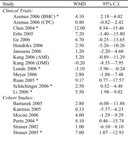
[image:3.595.306.514.201.430.2]The majority of the studies showed that BMC might bring beneficial effects to patients suffering from AMI and chronic IHD (WMD>0). Only two studies that involved a smaller number of subjects showed a different result (WMD≤0; Table 1).
Table 1: Reported Observed Study-Effects
Study WMD 95% C.I.
Clinical Trials:
Assmus 2006 (BMC) * 4.10 2.18—6.02 Assmus 2006 (CPC) 0.80 -0.82—2.42 Chen 2004 * 12.00 8.54—15.46 Erbs 2005 7.20 -1.40—15.80 Ge 2006 6.70 -0.25—13.65 Hendrikx 2006 2.50 -5.26—10.26 Janssens 2006 1.20 -2.20—4.60 Kang 2006 (AMI) 5.20 -0.89—11.29 Kang 2006 (OMI) -0.20 -8.35—7.95 Lunde 2006 * -3.10 -5.96— -0.24 Meyer 2006 2.80 -1.88—7.48 Ruan 2005 * 9.17 0.77—17.57 Schächinger 2006 * 2.50 0.52—4.48 Li 2006 * 5.50 1.98—9.02
Cohort Studies:
Bartunek 2005 2.80 -6.08—11.88 Katritsis 2005 0.33 -5.57—6.23 Mocini 2006 4.00 -1.29—9.29 Perin 2004 * 8.10 0.46—15.74 Strauer 2002 1.00 -6.10—8.10 Strauer 2005 * 7.00 1.07—12.93
* Statistically significant
Combining all 14 clinical trials and 6 cohort studies, the conventional random-effect meta-analysis suggests that BMC transplantation improved LVEF by about 4% (95% C.I.: 2.49—5.53). The results are reported in Table 2a. Thus, there seems to be sufficient evidence suggesting that patients on BMC showed modest improvement in LVEF when compared with the controls. The choice of a random-effect model is justified with the test for heterogeneity (p<0.001).
The Bayesian models with different priors were built next. Different prior values for θ reflect the different beliefs of the effects of BMC when compared with the controlled group. The prior for τ, however, was standardised as Gamma[λ: 0.01, η: 0.01] in all Bayesian analyses. The choice of this distribution reflected the lack of prior evidence regarding between-study precision. Also, the number of burn-ins was set a priori at 500 and the Markov chain would thereafter be run another 1,000 times before the final analyses (posterior) were reported.
In the second attempt, an optimistic prior was applied again. However, it is an “non-informative” prior with low precision, i.e., Normal[μ: 1.00, ν: 0.00001]. Resembling a flat or heavy-tailed distribution, this diffuse prior is effectively a uniform distribution which suggests that there was little prior information regarding θ at the time when the analysis was conducted. It is expected that such diffuse prior could cause little impact on the posterior. The combined effect turned out to be 3.96 (95% C.I.: 2.31—5.61; Table 2c). As readily seen, the combined posterior effect is very similar to that reported in the conventional analysis (Table 2a). The fairly wide interval estimate was a result of the inclusion of two non-informative priors.
In the next exploratory Bayesian analysis, a prior suggesting that there was no beneficial BMC effect was fitted. In this case, the “indifferent” prior for θ was chosen as Normal[μ: 0, ν: 10]. As shown in Table 3d, the combined effect turned out to be 0.30 and the associated 95% C.I. was -0.29—0.89. As a result, one may interpret that BMC did not bring significant benefits to the patients as the 95% C.I. contains zero.
To further illustrate the properties of the proposed Bayesian model, an “non-informative indifferent” prior with low precision was fixed next, i.e, Normal[μ: 0, ν: 0.00001]. The result was identical to the previous analyses based on “optimistic but weak” prior (Tables 2c-d), which in turn similar to the conventional analysis (Table 2a).
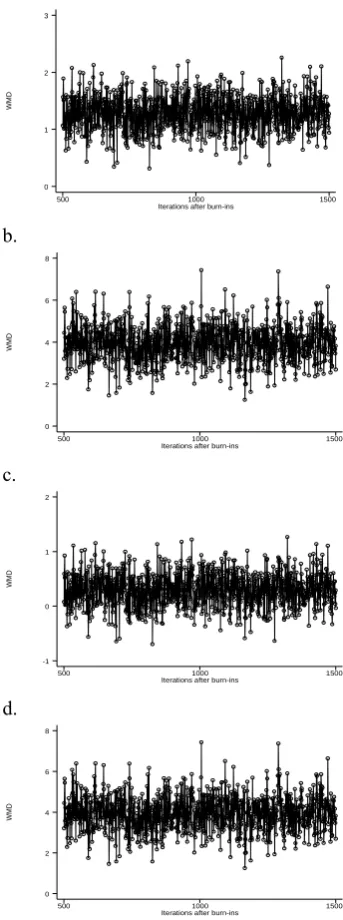
[image:4.595.309.481.71.532.2]In passing, note that the resultant posteriors based on the 4 different sets of priors were fairly normal and the Markov chains exhibited no obvious pattern of divergence after the burn-in values had been discarded (Figure 1).
Table 2: Results of Conventional and Bayesian Models
Models Combined Effect
(Posterior WMD)
95% C.I.
a. Conventional Random Model 4.01 2.49—5.53 b. Bayesian Meta-Analysis:
Optimistic but Strong Prior (in favour of BMC) Prior Effect: 1.00
Prior Precision of Effect: 10
1.29 0.70—1.87
c. Optimistic but Weak Prior (in favour of BMC) Prior Effect: 1.00
Prior Precision of Effect: 0.00001
3.96 2.31—5.61
d. Indifferent but Strong Prior Prior Effect: 0
Prior Precision of Effect: 10
0.30 -0.29—0.89
e. Indifferent but Weak Prior Prior Effect: 0
Prior Precision of Effect: 0.00001
[image:4.595.46.295.452.648.2]3.96 2.31—5.61
Figure 1: Iterative History of Bayesian Models a.
WM
D
Iterations after burn-ins
500 1000 1500 0
1 2 3
b.
WM
D
Iterations after burn-ins
500 1000 1500 0
2 4 6 8
c.
WM
D
Iterations after burn-ins
500 1000 1500 -1
0 1 2
d.
WM
D
Iterations after burn-ins
500 1000 1500 0
2 4 6 8
IV. DISCUSSION/CONCLUSION
The Bayesian meta-analysis model developed in this paper differs from the conventional approach in two aspects. First, it allows prior information—in the form of expert opinion and published evidence—to be incorporated into analysis. From the methodological point of view, it is costly to ignore such information if available. Second, the analysis is conducted on the posterior distribution which summarises all the information, both prior- and data-based, that the analysts have about the unknown parameters.
Consequently, it is naïve to assume that study heterogeneity does not exist even with the support of formal statistical tests. Moreover, such statistical tests may lack power in detecting the underlying differences among studies. It is very rare for biomedical studies of the same objective/nature to be exactly comparable.
The proposed Bayesian model may also be called a hierarchical model because, loosely speaking, more than one level of prior and likelihood is specified. In this case, a particular observed quantity depends on an unknown parameter, which in turn follows a second-stage prior. This sequence of priors and parameters constitute a model with an extended or hierarchical data structure.
The above review based on Bayesian models share a very important common feature. The posteriors were dominated by their respective priors. This was the result of a “weak” likelihood. The majority of the selected studies showed that while there could be beneficial effects associated with BMC, the results were not statistically significant as the 95% C.I.s contained zero (Table 1). With a relatively “weak” likelihood, the posterior result would be strongly influenced by the prior, i.e., the combined posterior were largely similar to the priors. However, this point was not explicitly highlighted by the conventional meta-analysis model. In this case, the Bayesian analyses revealed more details of the collected data under study.
As a result, while the paper agrees with the current meta-analysis that “BMC transplantation in patients with acute MI and chronic IHD is associated with modest improvements in LVEF” [3], it is crucial to emphasise that the effect could turn out to be statistically non-significant as the posterior result was heavily influenced by the selected priors. More studies must be conducted before the final chapter is written.
Finally, it is worthwhile to make some suggestions regarding the elicitation of prior distributions for future research. In practice, one may form a “community” of prior distributions with inputs from a number of experts. Inferences may then be based on a consensus of the posterior results or a “final” prior may be formed by averaging the prior distributions elicited from the experts. Alternatively, one may also consider constructing a primary prior distribution and a number of similar priors that belong to the same class.
By offering an alternative perspective in meta-analysis, the proposed Bayesian model is expected to provide more insights and relevant solutions to existing biomedical problems. In fact, one may view the conventional model as a special case within the broader framework of Bayesian methodology.
ACKNOWLEDGMENT
We are grateful to Dr Kenneth Ng, former consultant cardiologist, Tan Tock Seng Hospital Pte Ltd, for introducing us to this interesting topic. Special thanks go to the authors of the original article cited and reviewed in this paper. They deserve commendations for conducting the first systematic review and meta-analysis on the topic. We would also like to express our heartfelt thanks to Mr I. White, Medical Research Council Biostatistics Unit, Institute of Public Health, University of Cambridge, for sharing with us the Bayesian framework for meta-analysis.
REFERENCES
[1] R. DerSimonian, and N. Laird, “Meta-analysis in Clinical Trials,”
Controlled Clinical Trial, vol. 7, 1986, pp. 177-188.
[2] J.L. Fleiss, “The statistical basis of meta-analysis,” Statistical Methods in Medical Research, vol. 2, 1993, pp. 121-145.
[3] A. Abdel-Latiff, R. Bolli, I.M. Tleyjeh, V.M. Montori, E.C. Perin, C.A. Hornung, E.K. Zuba-Surma, M. Al-Mallah M, and B. Dawn, “Adult bone marrow-derived cells for cardiac repair: a systematic review and meta-analysis,” Archives of Internal Medicine, vol. 167, 2007, pp. 989-997.
[4] T. Bayes, “An essay towards solving a problem in the doctrine of chance,” in Bayes’s Theorem, R. Swinburne, Ed. Oxford: Oxford
University Press, 2002.
[5] S. Chib, and E. Greenberg, “Understanding the Metropolis-Hastings algorithm,” Annals of Mathematical Statistics, vol. 49, 1995, pp. 327-335.
[6] S.P. Brooks, “Markov chain Monte Carlo method and its application,”
Statistics, vol. 47, 1998, pp. 69-100.
[7] B.P. Carlin, A. Gelman, and R.M. Neal, “Markov chain Monte Carlo in practice: a roundtable discussion,” Journal of the American Statistical Association, vol. 52, 1998, pp. 93-100.
[8] G. Casella, and E.I. George, “An introduction to Gibbs sampling,”
Annals of Mathematical Statistics, vol. 46, 1992, pp. 167-174. [9] A. Zellner, and C-K. Min, “Gibbs sampler: convergence criteria,”