Abstract—Electro-optical system that combines the advantages of optical and electronic system has been widely applied in signal processing. Because of advantages of real-time, parallel operation capability, and programmable flexibility, it is especially utilized in the pattern recognition, e.g., military radar system, secure entry system, biomedical detection, and many other applications. Moreover, color is one of the most significant and powerful visual information. Improving the JTC for polychromatic pattern recognition is a novel topic. Deutsch proposed a multi-channel single-output JTC. It is based on RGB color model and separates the color pattern into red, green, and blue components respectively and then displays on the spatial light modulator (SLM). Thereafter, RGB become a popular model to perform pattern recognition. However, it is known that red, green, and blue components are correlated with one another. Furthermore, there are some cases in which the use of the RGB chromatic system is not appropriate for obtaining effective polychromatic object recognition, e.g., RGB decomposition is not appropriated for discriminating between similar color objects. Therefore, we propose a novel nonzero order JTC based on ATD color model to achieve polychromatic pattern recognition. ATD color model is constituted by achromatic, tritanopic, and deuteranopic systems. People consider that ATD color model is the most to be close to human eyes. In this paper, we apply ATD color model to multi-channel nonzero order joint transform correlator and perform pattern recognition. To estimate whether ATD color model is suitable for pattern recognition, we compare with RGB, which is common used to perform pattern recognition. The terms of estimation contain recognition ability of rotational distortion, brightness performance, multi-level quantized reference functions, noise tolerance ability, and relationship between channels and channels. We utilize peak to correlation energy, peak to sidelobe ratio, correlation peak intensity, and mutual correlation coefficient as our performance evaluation parameters. Finally, the results show that ATD color model is suitable for pattern recognition.
Index Terms—joint transform correlator, pattern recognition, ATD.
I. INTRODUCTION
In the optical pattern recognition systems, VanderLugt correlator (VLC) [1] proposed by VanderLugt in 1964 and
Manuscript received December 30, 2008. This work was supported by the National Science Council in Taiwan, under Grant No. NSC 96-2628-E-155-005-MY3.
Chiehpo Chang is with the institute of Electro-Optical Engineering, Yuan Ze university, 135 Yung Tung Road, Taoyuan 32026, Taiwan.
Chulung Chen is with the institute of Electro-Optical Engineering, Yuan Ze university, 135 Yung Tung Road, Taoyuan 32026, Taiwan. (Corresponding author. Phone: +886-3-4638800 ext 7513; Fax: +886-3-4639355; E-mail: [email protected]).
Tengwen Chen is with the institute of Electro-Optical Engineering, Yuan Ze university, 135 Yung Tung Road, Taoyuan 32026, Taiwan.
Tiengsheng Lin is with the institute of Electro-Optical Engineering, Yuan Ze university, 135 Yung Tung Road, Taoyuan 32026, Taiwan.
joint transform correlator (JTC) [2] proposed by Weaver and Goodman in 1996 are most to be well-known. The VLC based systems and the JTC systems use Fourier domain filter and spatial domain filter respectively. However, the VLC needs to be accurate aligned along the optical axis. This is a tight condition. Accordingly, the JTC does not have this problem, it arranges the reference and the target pattern side by side in the same plane. Therefore, the JTC has become an attractive pattern recognition system during the past decade [3]–[5]. However, the classical JTC is not a perfect system, it still has many drawbacks needed to be improved, e.g., non-real-time, and large zero order term (or auto-correlation).
Yu and Lu utilized liquid crystal light value (LCLV) to replace the conventional negative of photo in 1984 [6]. They has been realized a real-time improvement of the JTC. In 1988, Javidi proposed a binary JTC [7]. The JTC is easily to achieve the real-time capability.
To remove the zero order term, in 1997, Lu et al. utilized the phase-shifting technique [8] and achieve the nonzero order JTC (NOJTC). In 1998, Li et al. utilized the joint transform power spectrum (JTPS) subtraction strategy [9] to design NOJTC.
To yield sharp correlation peaks, Alam et al. proposed a fringe-adjusted JTC based on Newton-Raphson algorithm [10]. They used fringe-adjusted filter (FAF) to reshape the JTPS and improve correlation discrimination. Furthermore, Mahalanobis et al. proposed a minimum average correlation energy (MACE) method [11]. The MACE method is used in Fourier domain and could obtain shaper correlation peaks and smaller sidelobes in the output plane [12]. Recently, Chen et al. [13]–[16] proposed a multi-level quantized reference functions (MQRF). The MQRF is used in spatial domain and optimized in frequency domain with technique of Lagrange multipliers. Furthermore, the MQRF are suitable to current liquid crystal spatial light modulator (LCSLM) because of their limited dynamic range requirement.
II. ANALYSIS
ATD color model was developed by Guth [17], [18]. People consider that it is most close to human eyes. The neural information provides one achromatic and two polychromatic systems, which construct the second stage. The response characteristics of the second stage show linear transformations of the receptor absorption. If the model is restricted to experiments that measure threshold, increment threshold, and other small–step discriminations, utilizing the linear transformation is effective. The three components of the second stage are denoted by A, T, and D, where A refers to the achromatic (bright-dark) channel that can be considered as the luminance channel, T the tritanopic channel that corresponds to the opponent response red-green, and D the
Joint Transform Correlator Based on Color Human
Vision Model for Polychromatic Pattern Recognition
deuteranopic opponent channel that corresponds to the opponent response blue-yellow. Eq. (1) shows the linear transformation matrix from RGB color model.
0.5967 0.3654 0
0.9553 1.2836 0 , 0.0248 0 0.0483
A R T G D B = − − (1)
where R, G, and B are the three components from RGB color model.
Early, the architecture of classical joint transform correlator (CJTC) is single channel and used to perform monochromatic pattern recognition. To achieve color pattern recognition, Deutsch proposed multi-channel architecture. In this paper, we utilize this technique to develop NOJTC. Fig. 1 is the architecture of multi-channel NOJTC. Multi-channel NOJTC consists of one laser, one spatial filter, one collimated lens (CL), one beam splitter (BS), one computer, two LCSLMs, two Fourier lens (FL), and two CCDs. In the beginning, we obtain the reference image and separate the target image into A, T, and D color components. Then, put the reference and target images in LCSLM1. Next, coherent laser pass through spatial filter. When the collimated light coming out of LCSLM1 pass through FL1, input information will be transformed into Fourier domain. Then, The CCD1 records the JTPS. After removing zero order term, the JTPS recorded by CCD1 will be sent to LCSLM2. When another collimated light coming out of LCSLM2 pass through FL2, JTPS will be inverse Fourier transformed. Finally, we can obtain the cross-correlation output without zero order term in CCD2. We describe the positions of reference and target images in Eq. (2).
3 3
0 0
1 1
( , ) m( , m) n( , n),
m n
i x y r x x y y t x x y y
= =
=
∑
+ + +∑
− + (2)where x0=b, y1=-a, y2=0, y3=a, rm(−x0,−ym) represent three color components and positions of reference functions (m=1,2,3 or A,T,D), t xn( ,0 −yn) represent three color components and positions of target image (n=1,2,3 or a,t,d). After the collimated light coming out of LCSLM1 pass through FL1, ( , )i x y will be Fourier transformed as Eq. (3).
3 0 1 3 0 1
( , ) ( , ) exp[ 2 ( )]
( , ) exp[ 2 ( )].
x y m x y x y m
m
n x y x y n
n
I f f R f f j f x f y
T f f j f x f y
π π = = = + + − +
∑
∑
(3)Joint transform power spectrum (JTPS) will be detected by CCD1 as follows:
{
}
2 3 2 0 1 2 3 0 1 3 3 * 0 1 1 * 0( , ) ( , ) exp 2 ( )
( , ) exp 2 ( )
( , ) ( , ) exp 2 2 ( ) ( , ) ( , ) exp 2 2
x y m x y x y m
m
n x y x y n
n
m x y n x y x y m n
m n
m x y n x y x y
I f f R f f j f x f y
T f f j f x f y
R f f T f f j f x f y y
R f f T f f j f x f
π π π π = = = = = + + − + + + − + − +
∑
∑
∑∑
{
}
3 3 1 1( m n) ,
m n y y = = −
∑∑
(4)where the symbol * denotes the complex conjugate. If we remove zero order term, cross-correlation output will be displayed in CCD2 as follows:
3 3
1 1
3 3 *
1 1
( , ) ( , ) ( 2 , )
( , ) ( 2 , ),
ij i j
i j
ij i j
i j
o x y c x y x b y a a
c x y x b y a a
δ δ = = = = = − − ⊗ + − + + ⊗ − + −
∑∑
∑∑
(5)where a1=a, a2=0, a3= −a, c x yij( , )=r x yi( , )t x yj( , ), the symbols and ⊗ denote the correlation and convolution
operations respectively.
Although we remove zero order term, the system is still weak in distortion invariance, e.g., rotation, scaling, etc. To overcome this drawback, a special reference function named minimum average correlation energy (MACE) is proposed to solve various distortions and to reduce the correlation sidelobe intensity are main advantages of MACE.
We assume that there are N centered training images spanning the desired distortion-invariant feature range;
( , ) m
r x y and tmi( , )x y represent the reference and i-th training images in the input respectively; m denotes one of the ATD channels. The useful Fourier transform pair can be shown as follows:
1
( , )
( , ) ( , ) ( , ) ( , ),
mi
m mi m x y mi x y
c x y
r x y t x y − R f f T f f
ℑ ∗ ℑ = (6)
where the symbol ℑ and ℑ−1 denote Fourier transform and
inverse Fourier transform respectively, cmi( , )x y is the correlation output. The desired correlation peak value for each training image is described as follows:
(0, 0) ( , ) ( , ) .
mi m x y mi x y x y
c =
∫∫
R f f T∗ f f df df (7) We know that the total energy in the spatial domain is equivalent to the total energy in the Fourier domain from Parseval’s theorem. Therefore, the correlation energy is expressed as Eq. (8).(
)
(
)
(
)
(
)
2 2 * , , , , . mim x y mi x y m x y x y
c x y dxdy
R f f T f f R f f df df
=
∫∫
∫∫
(8)
On the other hand, Eq. (7) can be rewritten with matrix multiplication for all N training images as follows:
1 2 ˆ
ˆ ˆT [ (0, 0) (0, 0) (0, 0)]T ,
m m m m mN m
T R∗ = c c … c =S (9)
where the superscript T denotes the transpose operation. ˆTm
is a complex-valued data matrix whose i-th column is obtained by lexicographically (row by row) scanning
( , ) mi x y
T f f from left to right and from top to bottom; similar scanning of Rk leads to a column vector ˆRm. ˆSm is a column
ˆ ˆ ˆ ,T
ave m m m
E =R D R∗ (10) where Dˆm is a real-valued diagonal matrix whose diagonal entry is the average of Tmi( ,f fx y)2 with respect to all training images. Furthermore, the solution of Eq. (9) is not unique. To overcome this problem and achieve an optimum solution, we minimize Eave and satisfy the constraint in Eq. (9). We utilize
the advantage of Lagrange multipliers and obtain reference functions in the Fourier domain as follows:
1 * 1 1ˆ
ˆ ˆ ˆ [(ˆ )T ˆ ˆ ] .
m m m m m m m
R D T− T D T− − S∗
= (11)
Next, we would like to demonstrate that the inverse Fourier transform of reference function ˆRm is a real-valued function. Let ˆ 1 ˆ2
m
D− =B , where Bˆ is a real-valued diagonal matrix whose elements are the positive reciprocal square roots of
ˆ m
D . Subsequently, Eq. (11) can be rewritten as follows:
* 1ˆ
ˆ ˆ ˆ ˆ[(ˆ )T ˆ ˆ ˆ ] .
m m m m m
R =BBT T BBT − S∗ (12) Let ˆ ˆBTm= ˆP, then (12) can be rewritten as follows:
* 1ˆ
ˆ ˆ ˆ[(ˆ )T ˆ] .
m m
R =BP P P− S∗ (13) We can easily verify that the column vector ˆRmrepresents a Hermitian image in the Fourier domain when ˆSm is a real-valued matrix. Therefore, ˆrm is a real-valued reference function in the spatial domain. Finally, we rearrange ˆRm as a square matrix R f fm( ,x y). r x ym( , ) can be obtained by inverse Fourier transform of R f fm( ,x y).
{
}
1
( , ) ( , ) ,
m m x y
r x y = ℑ− R f f (14) where m represents A,T, or D color component.
Together with the concept of MACE optimization, Chen et al. proposed the concept of MQRF. In a real word, the target for recognition may suffer from some distortions, the MACE is therefore introduced. The MQRF is obtained by quantizing this function with finite levels. It is utilized in the proposed device. Furthermore, commercial LCD circuit is designed with digital IC technology. The transmittance is controlled with voltages and is therefore quantized. Finally, MQRF can be expressed as
1
[ ]
( , ) ( m( ,x y) 2 ),Q m
R
r x y Round
M f f
−
= ℑ (15)
where M is the maximum of 1[Rm(fx,fy)]
−
ℑ ; Q is the
amplitude quantization parameter; Round(K) function rounds
K to the nearest integer.
In this section, we will introduce several performance evaluations to estimate the ability of recognition. The criteria are defined as follows.
CPI is the correlation peak intensity at the correlation output plane. We define it as follows:
2
CPI=c(0, 0) . (16) PCE is defined as the ratio between desired correlation peak energy and total correlation energy. It can detect the sharpness of the correlation peak. It is given as follow:
2 2 , (0, 0) PCE= . ( , ) x y c c x y
∑
(17)According to Eq. (16), we know that the higher PCE is, the higher accuracy of target will be.
PSR is denoted as the ratio between primary peak energy and secondary peak energy. It is another important measurement criterion of pattern recognition. We express it as follows:
{
}
2 2 , (0, 0) PSR= ,max ( , ) x y
c
c x y
α ∈
(18)
where α={( , ) |x y x >2, y >2}. The higher PSR means the better ability for pattern recognition.
APCE is the average of PCE and APSR is the average of PSR. In some case, we should collect more data. We should average PCE and PSR. The results are expressed as follows:
2 2 1 , (0, 0) 1 APCE= , ( , ) N i i i x y c
N = c x y
∑
∑
(19)and
{
}
2 2 1 , (0, 0) 1 APSR= .max ( , ) N
i
i i
x y c
N c x y
α = ∈
∑
(20)The higher APCE is, the higher accuracy of target will be. The higher APSR means the better ability for pattern recognition. When we perform pattern recognition, pattern does not always keep perfect. It will suffer more or less noisy. We define SNR for a color pattern as follows:
3
2
1 1 1
2
( , ) Total signal power
SNR= ,
Total noise power 3 M N
i i m n
t m n
M N σ
= = =
=
× × ×
∑∑∑
(21)
where i is the channel, ti is the amplitude of input signal at
pixel (m, n), σ2 is the variance of each pixel, and M×N is the pixel number.
correlation is less between two channels. Mutual correlation coefficient is expressed as follows:
*
2 2
( , ) ( , )
,
( , ) ( , )
a x y b x y dxdy
a x y dxdy b x y dxdy
β =
∫∫
∫∫
∫∫
(22)where a(x, y) and b(x, y) represent two channels.
Apply mutual correlation coefficient to detect the target image before perform pattern recognition. We can decide what color models are suitable to use. This is a very useful technique.
III. NUMERICAL RESULTS
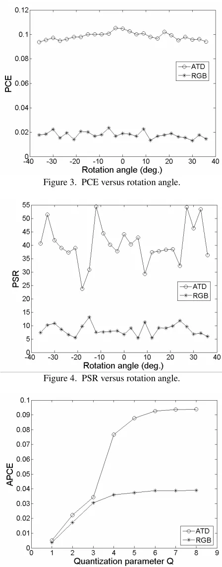
In the beginning, we pick a colorful butterfly pattern that comprises 128×128 pixels to be the original pattern. It is shown in Fig. 2. We rotate the original pattern and select a rotational distortion range of −36° to 36° (in steps of 3°). This training set contains 25 patterns. Table 1 presents the values of PCE, PSR, and CPI. Next, we plot the PCE and PSR versus different rotational distortion, as shown in Figs. 3, 4. In comparison with two models with different rotation angles, the performances on ATD color model is still better than RGB color model. The curve of PCE versus different rotation angles is smooth and steady for each training image. Notice the curve of PSR is oscillating and higher than certain level. We can see the recognition ability with ATD color model is better than that of RGB color model by above two measured criteria. Next, we will discuss the patterns with different intensities. Table 2 shows the measured criteria. Referring to table 1; we could observe that changes in PCE and PSR values are not much different. However, we know that it is a good recognition when CPI value is more over 50% of original value. When brightness is less than 50%, CPI value of RGB do not achieve 50% of original. Contraily, CPI value of ATD maintains more over 50% of original. The results imply that ATD color model is relatively independent of brightness. Fig. 5 shows the APCE versus different quantization parameters with ATD and RGB color models. We observe that the values of ATD and RGB increase quickly as the quantization parameter increases respectively from Q=1 to Q=4 and Q=1 to Q=3 and respectively slowly from Q=4 to Q=8 and from
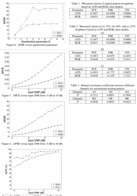
Q=3 to Q=8. Moreover, the value of ATD is higher than that of RGB from Q>3. Fig. 6 shows the APSR versus different quantization parameters. The situation is similar to that in Fig. 5. As a result, the saturation points of ATD and RGB are at quantization parameter Q=4 and Q=3, respectively. In real environment, the noise may affect this system and result in reducing recognition ability. For this reason, we test the performance for recognition by adding random Gaussian noise on the test image from -5 dB to 10 dB. In order to let the result be more accurate, we repeat 100 times at each SNR value. The numerical results of ACPI, APCE, and APSR versus SNR are shown in Figs. 7 to 9. The range of the SNR is from -5 dB to 10 dB. It is worthy to pay attention that ACPI is defined by noise-added CPI divides by noise-free CPI. Its unit is percentage (%). We can observe that the APCE values are quite close when SNR values are -5 dB to -3 dB. The variation of APCE values is getting larger and larger as SNR≥-3 dB.
The state of APSR curve is similar to that of the APCE curve. Moreover, the percentage of ACPI of RGB curve is higher than that of ATD curve, their values are over 50%. This shows that they all have enough recognition ability. Roughly, utilizing ATD color model to recognize is more suitable than RGB color model under noisy condition. Finally, table 3 shows the mutual correlation coefficients. It is obvious that the coefficients of RGB color model are higher than those of ATD color model. According to theorem, it means that RGB channels are highly correlated with one another. Therefore, ATD color model yields better effect.
IV. CONCLUSION
In this paper, we have proposed a multi-channel NOJTC based on a color human vision model named ATD color model. The main advantage of ATD color model is that it is the most to be close to human eyes. Therefore, the recognition results conform to the sense of sight of human. It will be helpful to research human eyes in the future.
According to the numerical results of comparison of discrimination capability of ATD and RGB color models, we verify that ATD color model could yield better recognition effect than RGB color model, e.g., rotation distortion, brightness performance, MQRF performance, noise tolerance ability, recognition ability of realistic background. Finally, the data of the mutual correlation coefficients also show ATD color model yield better effect. We know RGB color model is common utilized in image recognition field. Now, we show that ATD color model is also an alternative for pattern recognition. Since the concept of multi-channel is proposed and utilized in recognition, people try all kinds of color models to separate pattern into different channels. It is important that a suitable color model is required to match test pattern before the step of recognition. For the future works, we know that ATD color model is relatively independient of brightness; we could remove A channel and utilize TD two channels in recognition. On the other hand, we could find a technique to detect the test pattern and select a suitable color model.
REFERENCES
[1] A. VanderLugt, “Signal detection by complex spatial filtering,” IEEE Trans. Inf. Theory, IT-10, 139-145 (1964).
[2] C. S. Weaver and J. W. Goodman, “A technique for optically convolving two function,” Appl. Opt., 5, 1248-1249 (1996).
[3] X. J. Lu, F. T. S. Yu and D. A. Gregory, “Comparison of VanderLugt and joint transform correlator,” Appl. Phys., 51, 153-164 (1990).
[4] F. T. S. Yu, Q. W. Song, Y. S. Cheng and D. A. Gregory, “Comparison of detection efficiencies for VanderLugt and joint transform correlators,” Appl. Opt., 29, 225-232 (1990).
[5] P. Putwosumarto and F. T. S. Yu, “Robustness of joint transform correlator versus VanderLugt correlator,” Opt. Eng., 36, 2775-2780 (1997).
[7] B. Javidi and C. J. Kuo, “Joint transform image correlation using a binary spatial light modulator at the Fourier plane,” Appl. Opt., 27, 663-665 (198).
[8] G. Lu, Z. Zhang, S. Wu and F. T. S. Yu, “Implementation of a non-zero-order joint-transform correlator by use of phase-shifting techniques,” Appl. Opt., 36, 470-483 (1997).
[9] C. Li, S. Yin and F. T. S. Yu, “Nonzero-order joint transform correlator,” Opt. Eng., 37, 58-65 (1998). [10]M. S. Alam, X. Chen and M. A. Karim,
“Distortion-invariant fringe-adjusted joint transform correlation,” Appl. Opt., 36, 7422-7427 (1997). [11]A. Mahalanobis, B. V. K. V. Kumar and D. Casasent,
“Minimum average correlation energy filters,” Appl. Opt., 26, 3633-3640 (1987).
[12]C. Chen, “Minimum-variance nonzero order joint transform correlators,” Opt. Commun., 182, 91-94 (2000).
[13]C. Chen and J. Fang, “Cross-correlation peak optimization on joint transform correlators,” Opt. Commun., 178, 315-322 (2000).
[14]C. Chen, “Joint transform correlator with minimum peak variance in nonzero-mean noise environment,” Opt. Commun., 187, 319-323 (2001).
[15]C. Chen and J. Fang, “Optimal design of a nonzero order joint transform correlator with a real-valued reference function for distortion invariant fingerprint recognition,”
Opt. Memory and Neural Networks, 11, 45-54 (2002). [16]C. Chen and J. Fang, “Non-zero order joint transform
correlator with multi-level quantized reference function,”
Opt. Commun., 220, 41-47 (2003).
[17]S. L. Guth, R. W. Massof, and T. Benzschawel, “Vector model for normal and dichromatic color vision,” J. Opt. Soc. Am., 70, 197-212 (1980).
[18]S. L. Guth, “Unified model for human color perception and visual adapation,” Proc. SPIE, 107, 370 (1989). [19]C. Chen and W. Wu, “Color pattern recognition with the
[image:5.612.314.538.44.615.2]multi-channel non-zero-order joint transform correlator based on the HSV color space,” Opt. Commun., 244, 51-59 (2005).
Figure 1. Multi-channel NOJTC system.
Figure 2. Noise-free original pattern.
Figure 3. PCE versus rotation angle.
Figure 4. PSR versus rotation angle.
[image:5.612.138.230.638.729.2]Figure 6. APSR versus quantization parameter.
[image:6.612.72.547.41.720.2]Figure 7. APCE versus input SNR from -5 dB to 10 dB.
Figure 8. APSR versus input SNR from -5 dB to 10 dB.
Figure 9. ACPI versus input SNR from -5 dB to 10 dB.
Table 1. Measured criteria of orginal pattern recognition based on ATD and RGB color models.
Parameter PCE PSR CPI
ATD 0.1047 44.0980 9.0000
RGB 0.0431 16.6980 9.0000
Table 2. Measured criteria of (a) 75%, (b) 50%, and (c) 25% brightness based on ATD and RGB color models.
(a)
Parameter PCE PSR CPI
ATD 0.1047 44.0980 9.0000
RGB 0.0431 16.6980 9.0000
(b)
Parameter PCE PSR CPI
ATD 0.1057 44.879 6.2452
RGB 0.0448 16.076 2.9211
(c)
Parameter PCE PSR CPI
ATD 0.1053 41.772 5.0652
RGB 0.0436 11.429 1.1221
Table 3. Mutual correlation coefficients between different channels for unrotational training pattern.
Channels AT TD DA
β 0.2713 0.0051 0.7890
Channels RG GB BR
[image:6.612.83.288.555.715.2]