Munich Personal RePEc Archive
Search and Ripoff Externalities
Armstrong, Mark
Department of Economics, University of Oxford
July 2014
Search and Ripo¤ Externalities
Mark Armstrong
July 2014
Abstract
This paper surveys models of markets in which some consumers are “savvy” while others are not. We discuss when the presence of savvy consumers improves the deals available to non-savvy consumers in the market (the case of search externalities), and when the non-savvy fund generous deals for savvy consumers (ripo¤ externalities). We also discuss when the two groups of consumers have aligned or divergent views about market interventions. The analysis covers two overlapping families of models: those which examine markets with price/quality dispersion, and those which exhibit forms of consumer hold-up.
Keywords: Consumer protection, consumer search, price dispersion, hold-up, add-on pricing.
1
Introduction
This paper examines a number of situations in which “savvy” and “non-savvy” consumers
interact in the marketplace. An old intuition in economics suggests that savvy consumers
help to protect other consumers, and that consumer policies which protect vulnerable
consumers are only needed when there are insu¢cient numbers of savvy types present in the market. In broad terms, a “search externality” operates so that those consumers who are
better informed about the deals available in the market ensure that less informed consumers
also obtain reasonable outcomes. Recent work, however, has examined situations where
savvy consumers bene…t from the presence of non-savvy types. In such markets, a “ripo¤
externality” is present, and vulnerable consumers may need protection even when they are
small in number.
This paper discusses three principal issues. First, what kinds of inter-consumer exter-nalities are present? That is, when do savvy consumers protect other consumers, when do
non-savvy consumers improve the deals o¤ered to the savvy, or when is there no interaction
between the two groups at all? Second, which kinds of market intervention bene…t both
consumer groups and which policies bene…t one group at the expense of the other? Third
and …nally, what determines the extent of savviness in the consumer population?
For our purposes, there are two broad notions of savviness to consider. First, a consumer
might be well informed about the prices and/or product qualities available in the market. For instance, a savvy consumer shopping for wine is able to determine the likely quality
of the wine inside by looking at the label. Alternatively, a consumer looking for a new television may know the range of available prices (e.g., because she is online), or knows how
much she is willing to pay for a product before travelling to the seller. Second, a consumer
might bestrategically savvy, in that she has a good understanding of the game being played in the market. For instance, consumers might be unable to discern product quality (i.e.,
they are non-savvy in the …rst sense) but they understand how quality depends on price in
equilibrium and buy accordingly. Or they might foresee a …rm’s incentive to set its future
prices. A consumer who is savvy in this sense is aware of her future behaviour, while a
strategically naive consumer might not predict accurately how she will behave.
A consumer might be non-savvy in both senses. For instance, she might not be able to
discern quality and also might not foresee how quality depends on price. Indeed, strategic
naivety might be the cause of information problems. For instance, in a market where in
fact there is price dispersion, but naive consumers think that all sellers o¤er the same price,
a naive consumer might choose not to incur search costs to become informed about the
prices in the market.
A useful framework for discussing the issues is the following.1 Suppose there are two
kinds of consumers, “savvy” and “non-savvy”, and the proportion of savvy consumers in
the population is . To focus on the impact of savviness on outcomes, we suppose that there are no systematic di¤erences in tastes for the product in question across the two groups of consumers. Except for section 2.2, we take the extent of savviness, , to be
exogenous and out of the control of consumers and …rms.
Let VS( ) and VN( ) denote the expected net surplus enjoyed in equilibrium by an
individual savvy and non-savvy consumer respectively, whileV( ) VS( )+(1 )VN( )
measures aggregate consumer surplus. We expect that VS( ) VN( ), so that savvy
consumers obtain better deals than their non-savvy counterparts.2 This is because tastes
do not di¤er across the two groups of consumer, and a savvy type could mimic a non-savvy
buying strategy and so obtain surplusVN. A rational, but uninformed, buyer must obtain
non-negative surplus VN 0, for otherwise she would choose to stay out of the market.
However, a strategically naive consumer might experience negative surplus. In many cases
VS and VN move the same way with —i.e., either both increase with , both decrease
with , or neither depends on —although it is not inevitable this be so.3
Likewise, let S( ) and N( ) denote the pro…t generated in equilibrium by an
indi-vidual savvy and non-savvy consumer respectively, while ( ) S( ) + (1 ) N( )
measures industry pro…t. Here, it is less clear how S and N compare, although in most
of the situations discussed in this paper non-savvy consumers generate more pro…t than
the savvy and S( ) N( ). In perfectly competitive situations, we expect all pro…ts
to be zero. Finally, let W( ) V( ) + ( ) denote total welfare.
There are (at least) three cases of interest:
Search externalities: When savvy consumers exert a positive externality on the non-savvy—that is, when VN( ) increases with —we say that “search externalities” are
present. This is because the leading example where savvy consumers protect non-savvy
consumers is when the former are better informed about prices or qualities available in the
market, and when there are more consumers aware of all the available deals this makes
suppliers o¤er good deals, which in turn are available to more inert buyers.4 As we will see, within this class of markets, VS usually also increases with , while overall welfare W can
increase or decrease with and pro…ts might increase, decrease or be “hump-shaped”
in , depending on the context.
Ripo¤ externalities: When savvy consumers bene…t from the presence of the non-savvy—
2However, there are situations in which replacing a population of savvy buyers with a population of
non-savvy buyers will make buyers better o¤. For instance, this is the case in one of the hold-up scenarios discussed in section 3.1. There are also cases where the two kinds of consumer obtain exactly the same surplus; for example, this is often the case when a monopolist o¤ers a single product at a single price and so all consumers obtain the same deal.
3For instance, in section 2.3 the surplus enjoyed by savvy consumers can be a non-monotonic function
of , although non-savvy surplus increases with . Likewise, in the model of “bill shock” in section 3.2, it is possible thatVN increases with whileVS decreases with .
4At the time of writing this, the front-page headline of the UK’sDaily Telegraph on 9 July 2014 was
whenVS( ) decreases with —we say “ripo¤ externalities” are present. A leading example of this situation is when non-savvy consumers can be “ripped o¤” with extra charges, and
the resulting revenue is passed back to all consumers in the form of subsidized headline price. Another example of such a market (not discussed further in this paper) is Akerlof
(1970)’s lemons market, where savvy consumers who understand adverse selection can
cause the market to shut down. Strategically naive consumers, however, who mistakenly
believe the pool of products o¤ered for sale is una¤ected by the selling price—and who
may therefore pay more than the product is really worth to them—can allow the market to
open.5 In markets with ripo¤ externalities, it is possible that aggregate consumer surplus
V rises with , even if both VS and VN fall with , if the gapVS VN is large.
No interactions between consumers: On the knife edge between these two cases are situ-ations in which there is no interaction between the two groups of consumers, and VS and
VN do not depend on . These cases typically involve biased beliefs on the part of naive
consumers. If present, competition delivers what each type of consumer thinks they want,
and neither wishes to choose the deal o¤ered to the other type. Ex post, though, biassed consumers might regret the deal they chose. (A lucky charm which is sold to help predict
winning lottery numbers, say, has no impact on the savvy consumers who do not buy it,
but may be attractive ex ante to naive consumers.)
The plan for the rest of this paper is as follows. Oligopoly models which generate
price or quality dispersion are examined in section 2, and we will see that the search
externality tends to operate in such markets, so that savvy types confer a bene…t to the
non-savvy (and usually to other savvy types too). Models with various forms of “hold-up”
are presented in section 3, including situations with both an indivisible good and with a
more complex product involving add-on services.6 In these markets a richer set of outcomes
are possible, and seemingly minor variants of the add-on price problem generate each of
the three situations—search externalities, ripo¤ externalities, and no interaction—listed
above. We end the paper with some concluding comments.
5See Spiegler (2011, section 8.3) and the references listed there for further discussion of markets when
consumers have limited understanding of adverse selection.
6There is some overlap in the two classes of model. The model of quality dispersion in section 2.4 could
2
Price and Quality Dispersion
2.1
A model of price dispersion
In a market for an indivisible good of known quality, it is intuitive that when some
con-sumers are aware of available prices and buy from the cheapest supplier, those who shop less diligently are partially protected.
To illustrate this, consider Varian (1980)’s classical model of price dispersion.7 Here,
n identical …rms supply a homogeneous product with unit cost c. In general, consumers
di¤er in their reservation value for the item,v, where the fraction of consumers withv p
is denotedq(p). For ease of notation, write (p) (p c)q(p)for pro…t with pricep, which
we assume is quasi-concave in p, and pM for the price which maximizes this pro…t. An
exogenous fraction of consumers (independent of the valuationv) are savvy, in the sense
that they buy from the cheapest supplier, while other1 consumers buy from a random
supplier so long as that supplier’s price is below their v.8
In cases where all consumers are savvy or all are non-savvy, there is a pure strategy
equilibrium and no price dispersion. If = 1, so that all consumers shop around, there is
Bertrand competition and price is driven down to cost c. If = 0, so that all consumers
shop randomly, then no supplier has an incentive to set price below the monopoly price
pM, and the outcome is as if a single …rm supplied the market. Since there is no price
dispersion, it follows that VN = VS and N = S in these extreme cases. (Here, V and
refer to the expected value of a consumer’s surplus and pro…t, with expectations taken
over the idiosyncratic valuationv.)
However, in a mixed market with 0 < < 1, the only (static) equilibrium involves a mixed strategy for prices, so there is price dispersion in the market and a savvy consumer
obtains a (weakly) lower price than any non-savvy consumer. It follows thatVS > VN and
S < N. In more detail, the symmetric equilibrium involves each …rm choosing its price
according to a cumulative distribution function (CDF) F(p), which satis…es
(1 F(p))n 1 + 1
n(1 ) (p) 1
n(1 ) (p
M) : (1)
7See Salop and Stiglitz (1977) for closely related analysis.
8This behaviour could be justi…ed if each consumer’s cost of search is very convex, in the sense that a
Here, a …rm which chooses price p will sell to all savvy consumers (who have v p) provided all of its rivals choose a higher price, which occurs with probability(1 F(p))n 1
in this equilibrium. On the other hand, the …rm will always sell to its share of the1 inert
consumers (who havev p). As such, a …rm’s demand from the uninformed consumers is
less elastic than demand from the informed. The left-hand side of (1) is therefore the seller’s
pro…t if it sets price p. Since the seller could decide only to serve its captive consumers,
who are 1
n(1 ) in number, with the monopoly price, the right-hand side represents a
seller’s available pro…t.9 For a …rm to be willing to play the mixed strategy F( ), the …rm
must be indi¤erent between all prices in the support of F( ).
The value of F(p) which solves (1) is an increasing function of . That is, when the fraction of savvy consumers is higher, each seller is more likely to set low prices. Intuitively,
increasing makes a seller’s demand more elastic. Because each seller’s price distribution
is shifted downwards (in the sense of …rst-order stochastic dominance) when rises, both
the savvy consumers (who pay the minimum price fromn draws) and the inert consumers
(who pay the price from a single draw) are better o¤ when is higher. In the notation of
section 1, then,VS andVN increase with , as does aggregate consumer surplus. From (1),
industry pro…t is ( ) = (1 ) (pM), which decreases with . Total welfare W at least
weakly increases with since lower prices stimulate demand.
0.0 0.1 0.2 0.3 0.4 0.5 0.6 0.7 0.8 0.9 1.0 0.0
0.2 0.4 0.6 0.8 1.0
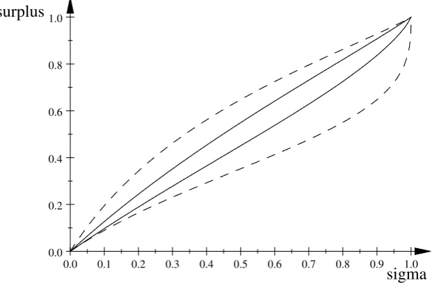
[image:7.595.148.459.469.674.2]sigma surplus
Figure 1: Expected surplus with price dispersion (n= 2 and n = 4)
9However, it is not an equilibrium for sellers to choose the monopoly price p= pM
Figure 1 depicts the net surpluses VS and VN enjoyed by the savvy (the upper solid
curve) and the inert (lower solid curve) consumers when all consumers are willing to pay
v = 1 for the item and c = 0, so that (p) = p if p 1, and when n = 2. Note that
the extent of price dispersion, as captured by the gap between the minimum and average
price in the market, is non-monotonic in . (As discussed, there is no price dispersion
when = 0 or = 1.) As such, increasing might increase or decrease the extent of price
dispersion in a market, depending on the initial level of savviness.10
The two solid curves on Figure 1 are rather close together, indicating there is a limited
bene…t to a consumer in knowing both prices. When the number of suppliers is larger,
however, one can show that the expected price paid by savvy consumers falls while the expected price paid by the inert shoppers rises, so the two curves on Figure 1 move further
apart. Intuitively, a …rm’s demand from the savvy consumers, (1 F)n 1
, falls with n
faster than its demand from the inert, (1 )=n, and so with larger n a …rm puts more
weight on extracting revenue from the latter group. (One can see that the prices paid by
informed and uninformed consumers must move in opposite directions asn increases, since
industry pro…t ( ) = (1 ) (pM)does not depend onn.) The dashed lines on the …gure
show the respective surplus functions in this example when n = 4. Thus, increasing the
number of suppliers has contrasting e¤ects on the informed and the uninformed consumers, with only the savvy bene…tting from “more competition” of this form.11
Extension to this benchmark model:
A modi…cation to the above model allows suppliers to charge distinct prices to savvy and
inert consumers. For example, the former group might be those who use a price-comparison
website and buy online, while the uninformed go to a random bricks-and-mortar store, and
a supplier might set di¤erent prices for the two purchase channels. When this form of
price discrimination is used, the link between the two groups is broken, and the outcome
is that the informed consumers are o¤ered a low price equal to marginal cost c, while the
uninformed are charged the monopoly pricepM. In this case, there is no search externality
and the fraction of informed consumers has no impact on the surplus of either group.12
10Brown and Goolsbee (2002) …nd evidence consistent with this, when they observe that price dispersion
rises when the use of price comparison websites increases from a low level, then decreases as their use becomes more widespread.
11See Morgan, Orzen, and Sefton (2006) for further discussion of the impact of changing and n on
payo¤s to consumers. These authors also conduct an experiment, where human sellers face computer consumers, and which con…rms the model’s predictions quite closely.
A second variant of Varian’s model extends the analysis to a dynamic setting, and examines the impact of consumer savviness on the sustainability of tacit collusion in this
market.13 Suppose the industry attempts to collude at the monopoly pricepM with the use
of a trigger strategy. If a …rm deviates by undercuttingpM, suppose this is detected by all
rivals, and from the next period onwards the industry plays the one-shot Nash equilibrium
with mixed strategies described above, yielding per-…rm pro…ts in each period given by
the right-hand side of (1). If a …rm does undercut the collusive price, this lower price
is observed only by the savvy consumers. As a result, when is the discount factor,
collusion at the monopoly price can be sustained if
1 1
(pM)
n
| {z }
collusive pro…t
( + 1
n ) (p
M)
| {z }
deviation pro…t
+
1 (1 ) (pM)
n
| {z }
punishment pro…t
which reduces to the usual condition
n 1
n :
In this market, increasing has two contrasting e¤ects. When is large there is …erce
competition without collusion, and so the punishment pro…ts are small. On the other
hand, when is large, the number of consumers who respond to a price cut is large, and
so short-run gains from deviating are large. These two e¤ects precisely cancel out, and the
ability to collude is una¤ected by the number of savvy consumers.
A …nal variant considers a situation in which, instead of purchasing from a random
seller, a sales intermediary (or “salesman” for brevity) steers the inert consumers towards
a supplier of his choice, if given incentive by that supplier to do so. These naive consumers
follow sales advice, without understanding that the advice might be biassed by …nancial
inducements from sellers.14
website, and can charge di¤erent prices on this website and when they sell direct to consumers. They …nd that sellers choose whether to list according to a mixed strategy and choose their price on the comparison website according to a mixed strategy, and obtain positive pro…ts there generated by the possibility they are the sole listing seller. The price on the comparison website is lower than its price on its own platform. 13See Schultz (2005) for this analysis, as well as its extension to a market with horizontally di¤erentiated
products. Petrikaite (2014) analyzes an alternative model in which consumers can become informed about prices and valuations by incurring a search cost. She …nds that in an increase in this search cost—i.e., a reduction in market transparency—makes collusion easier to achieve.
14Inderst and Ottaviani (2012, page 502) report how a majority of people who had received …nancial
In more detail Armstrong and Zhou (2011, section 1) suppose that a number of sym-metric suppliers costlessly supply a homogenous product which all consumers value at v.
This product is only available via a consultation with a salesman. An exogenous
frac-tion of savvy consumers are immune to the salesman’s patter, costlessly observe the full
list of retail prices, and buy from the cheapest supplier. The remaining fraction 1
of consumers are susceptible to the marketing e¤orts of the salesman and follow his
rec-ommendation. Suppose that a supplier chooses its retail price, p, and commission rate, b,
simultaneously (and simultaneously with its rivals). In this setting a salesman will promote
the highest-commission product (regardless of how retail prices compare).
When = 1, so that all consumers are savvy, there is no point in a seller spending re-sources to in‡uence a salesman, and the result is Bertrand price competition, and suppliers
and salesmen obtain no pro…ts. When = 0, the salesman determines demand entirely,
and so suppliers compete to o¤er the highest commission. The result is that both the retail
price and the commission payment is driven up to v, so that suppliers obtain zero pro…t
but salesmen extract the entire social surplus. In either case, there is no price dispersion.
When 0< <1 sellers choose their retail prices and commission payments randomly.
In equilibrium, there is an increasing relationship between a …rm’s choice ofbandp. This is
because a higher pricepmakes it more worthwhile for a seller to pay the salesman to steer the uninformed consumers towards its product. Since high commissions are associated
with high retail prices, there is “mis-selling”, and a salesman promotes the more expensive
product due to the higher commission he receives. The expected outlay for a non-savvy
consumer is the expected value of thehighest of the retail prices in the market, rather than the the expected value of a random price in the market as in Varian’s model.
In the case with two suppliers, Armstrong and Zhou (2011) show there is a linear
relationship between a supplier’s price and its commission. Speci…cally, the lowest retail
price a supplier o¤ers ispmin = (1 )v, and if a supplier chooses retail pricepit will o¤er
a salesman the commission payment
b(p) = 1 (p pmin) :
As in Varian’s original model, one can show that the surpluses of savvy and non-savvy
consumers increase with , while the total pro…ts of suppliers and salesmen combined
decreases with .
commission payments. Suppose that salesmen remain necessary for consumers to buy the product, but commission payments are banned and a salesman is instead paid directly for a
consultation by consumers. Competition between salesmen implies that their consultation
charge is zero. Suppose that when a salesman receives no commissions, he steers the naive
consumers to the cheaper product. (This might be because, all else equal, he has a small
intrinsic preference for assigning the appropriate product to consumers.) In this case, all
consumers buy the cheaper product and in Bertrand fashion the sellers are forced to set
their retail prices equal to cost. It follows that both groups of consumers are better o¤ in
the no-commission regime (although salesmen and suppliers are worse o¤).15
2.2
The equilibrium number of savvy consumers
When consumers choose to be savvy
When information about market conditions and product attributes is costly to acquire,
it may be rational to stay uninformed, especially when the search externality is present
and most other consumers are already well informed.16 To discuss the equilibrium extent
of savviness, continue with the model of price dispersion from the previous section, and
when the fraction of savvy types is write a savvy consumer’s surplus as VS( ) and the surplus of an uninformed consumer as VN( ). (The following argument is easiest if we
assume all consumers have the same value v for the product, so that all consumers will
buy in equilibrium.) As illustrated on Figure 1, VS and VN increase with , and where the
incentive to become informed, VS( ) VN( ), is “hump-shaped” such thatVS(0) VN(0) =
VS(1) VN(1) = 0.
Suppose that consumers can switch from being ignorant to informed by incurring an
information acquisition cost, . In general, consumers may di¤er in their cost of acquiring
information, and let ( ) be the corresponding cost of the marginal consumer when
consumers choose to become informed. A consumer with information acquisition cost will choose to become informed if and only if VS( ) VN( ), and consumers will
choose to become informed until the marginal consumer is indi¤erent. Thus, the fraction
15Inderst and Ottaviani (2012) present an alternative model of mis-selling, where the salesman advises
consumers about the suitability of a product rather than its price. There, no consumers are informed, and must rely on the salesman to advise them about which product to buy. The salesman has only a noisy signal about the suitability of a product, and he has an intrinsic preference to recommend the suitable product to a consumer. However, this preference can be overturned if a seller sets a high enough commission.
16The issue of how many agents rationally decide to remain uninformed in a market equilibrium was
of consumers who become informed in an interior equilibrium with 0< <1satis…es
VS( ) VN( ) = ( ) : (2)
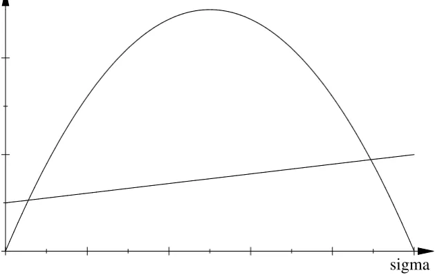
Figure 3 illustrates the equilibria, where the hump-shaped curve, VS( ) VN( ),
cap-tures the bene…t of being informed, while the upward-sloping line ( ) represents the cost
of becoming informed. The …gure shows there are two interior equilibria satisfying (8), a
low- and a high- equilibrium. However, only the high- equilibrium is “stable”, while at
the low- equilibrium a perturbation in will induce to move away from this point. As
emphasized by Grossman and Stiglitz (1980) in a related model, it is never an equilibrium
for all consumers to become informed. In any interior equilibrium, because of the search externality too few consumers choose to be informed—and too many prefer to free-ride on other consumers’ search e¤orts—and aggregate consumer surplus would be boosted if
were locally increased.17 (By contrast, if the market instead had a ripo¤ externality, in
the sense that aggregate consumer surplus was a decreasing function of , there would be
excessive numbers of consumers choosing to be savvy.)
[image:12.595.144.459.404.603.2]sigma
Figure 2: The fraction of consumers who choose to be informed
If (0) > 0, as depicted on the …gure, there is a second stable equilibrium where
= 0. When no one becomes informed, all consumers obtain the same (bad) deal in
17Formally, aggregate consumer surplus when consumers incur the cost of being informed is
VS( ) + (1 )VN( )
Z
0
(~)d~
the market, and there is no point investing in acquiring information to …nd a better deal. This equilibrium is akin to Diamond (1971)’s paradox. However, if a fraction of consumer
actively enjoy shopping, so that ( ) = 0for su¢ciently all small , the unique equilibrium
may be the high- equilibrium.
One can imagine consumer policies which a¤ect either the cost curve or the bene…t
curve. Assuming that it is the high- equilibrium which is relevant, a policy which reduces
information acquisition costs—in the sense of shifting the curve ( ) downwards—will
increase , and this will in turn bene…t all consumers. Likewise, a policy which shifts
the bene…t curve upwards will increase equilibrium . For example, in the model of price
dispersion in section 2.1, we saw on Figure 1 that increasing the number of suppliers pushed the surplus of the two groups of consumers further apart, and so shifted the bene…t curve
upwards. Since this will increase , it may be that increasing the number of suppliers will
in equilibrium bene…t all consumers once the impact on is taken into account.18
On the other hand, a policy which shifts the bene…t curve downwards will reduce the
fraction of consumers who choose to become informed.19 Consider the model of price
dis-persion discussed in section 2.1, specialized to the case with two sellers, consumer valuation
v = 1 and costless production as depicted on Figure 1. Suppose that any consumer can
become informed of both prices, rather than having to shop randomly, by incurring the cost = 1
20. In this case, a fraction 0:95 of consumers choose to be informed and all
consumers have expected outlay (including information costs where relevant) of about0:1.
In this example most consumers obtain what seems like a good deal, obtaining the item
in return for an outlay which is only 10% of their valuation. However, a few consumers
will pay up to ten times this price, and pressure—from the media, politicians, or consumer
groups—to protect consumers from these occasional high prices could arise. Suppose in
response that a new policy constrains …rms to set prices no higher than 1
2, so that the
max-imum permitted price is halved. For a given , the expected prices paid by the informed
and uninformed consumers then halve, and hence the incentive to become informed also
18To take an extreme example, if all consumers have information acquisition cost = 1
10, then by exam-ining Figure 1 we see that the only equilibrium with duopoly involves no consumers becoming informed, in which case all consumers are charged the monopoly price p = 1. However, with four suppliers, the maximum gap betweenVS andVN is greater than , and a stable equilibrium with 1 emerges where
all consumers have total outlay of about = 1
10. A contrasting e¤ect is discussed in Spiegler (2011, page 150). When a consumer is faced with a greater number of suppliers, she may su¤er from “choice overload”, with the result thatfewer consumers are savvy.
halves. The result is that the fraction of informed consumers falls to 0:74, so that the number of uninformed consumers rises about 5-fold as a result of the policy. Each
consumer now has expected outlay of about0:17, which is 70% higher than in the absence
of the price cap. Industry pro…t more thandoubles as a result of the imposition of the price cap. Thus, the perverse e¤ect of this well-intentioned consumer policy can be substantial.20
When …rms confuse consumers
The previous section discussed how consumers can take the initiative to become savvy.
Clearly, …rms also play role in suppling information to consumers, and there is a vast
economic literature about how …rms advertise their products and prices. Less familiar is the possibility that the …rms attempt to “confuse” consumers, with the result that the
fraction of savvy types falls. For example, …rms might present their prices in an opaque
way or in a di¤erent format to their rivals, and this makes it hard for some consumers to
compare deals.21
To illustrate this possibility, consider the following extension to the price dispersion
model of section 2.1.22 There are two …rms, and a …rm can present its price in one of two
formats. If …rms choose the same format, consumers …nd it easy to compare prices and all
choose to buy from the …rm with the lower price. However, if …rms choose distinct formats
a fraction 1 of consumers are confused and buy randomly (while the remaining are savvy enough to make an accurate comparison even across formats).
In this context, …rms choose both prices and formats according to a mixed strategy.
Since the format itself does not matter, only whether the formats are the same or not, a
…rm chooses the same CDF for its price, say F(p), regardless of its chosen format, and is
equally likely to choose either format. If one …rm chooses a particular format and price p,
20Knittel and Stango (2003) examine the credit card market in the United States in the period 1979–89,
during which usury laws in some states put a ceiling on permitted interest rates. In their Table 3 they show how, for much of this period, average interest rates werehigher in those states with a ceiling, and interpret this as evidence that price caps can encourage tacit collusion via a policy-induced focal point. The (static) search model presented in the text provides an alternative explanation for why a price cap might lead to price rises.
21For instance, Clerides and Courty (2013) observe empirically that the same brand of detergent is sold
in two sizes, the large size containing twice as much as the smaller. Sometimes the large size is more than twice as expensive as the smaller, and yet signi…cant numbers of consumers still buy it.
then as in expression (1) its expected pro…t is
0
@1
2[1 F(p)]
| {z }
same format
+1
2[ (1 F(p)) + 1
2(1 )]
| {z }
di¤erent format
1
A(p c) 1
4(1 )(v c):
Here, if the two …rms display their prices in the same format there is …erce competition,
and the cheaper …rm wins the whole market, while if the formats di¤er a fraction(1 )of consumer shop randomly. The right-hand side of the above represents the pro…t obtained
when a …rm happens to have a di¤erent format and fully exploits its captive consumers,
which is each …rm’s equilibrium expected pro…t.
It is not an equilibrium for …rms to choose their format deterministically. Clearly, if
both …rms were known to choose the same format, price would be driven down to cost and
pro…t to zero. In that case, a …rm could switch format to make money from the newly
confused consumers. If both …rms were known to choose distinct formats, prices would be
chosen according to a mixed strategy as in (1). However, in that case, a …rm could switch
to o¤er the same format as its rival and o¤er the lowest price in the price support, which ensures it serves the entire market and boosts its pro…t.
This model predicts that …rms engage in “tari¤ di¤erentiation” to obtain positive
prof-its, just as …rms in more traditional oligopoly models engage in product di¤erentiation.
However, unlike forms of product di¤erentiation, this tari¤ di¤erentiation confers no
wel-fare gains. A consumer policy which forced …rms to present prices in a common format
would, in this model, move the market to Bertrand price competition, and all consumers
would bene…t.23
2.3
Coasian pricing
Consider next a very di¤erent kind of model, the durable goods problem of Coase (1972).
There, a …rm sells its product over time to forward-looking consumers with heterogeneous
tastes for a single unit of its product. The …rm cannot commit to its future prices, and after
high-value consumers have purchased, the …rm has an incentive to reduce its price to sell to remaining lower-value consumers. This model can be viewed as an oligopoly market—
where the …rm “competes with itself” over time—with inter-temporal price dispersion.
23Additional features play a role when the two formats are “simple” and “opaque”, and when both …rms
(However, in contrast to the previous model, here price dispersion does not arise through the use of mixed strategies.)
We extend this classical model to allow a fraction 1 of consumers to be naive,
in the sense that they do not understand the …rm’s incentive to reduce its price over
time.24 As such, these naive consumers buy myopically, as soon as the price falls below
their valuation for the item. It follows that VN VS since naive consumers buy too
soon relative to the optimal purchasing strategy followed by the savvy, and since the …rm
obtains greater pro…t when a consumer buys more quickly we have N S. From this
perspective, naive consumers here are like the inert shoppers in Varian’s model (who can
be interpreted as mistakenly believing that all …rms o¤er the same price). The presence of these consumers tends to relax “intra-…rm” competition in Coase’s model, just as they
relax inter-…rm competition in Varian’s model, with the result that naive consumers are
protected by the presence of the savvy, while pro…ts are harmed. However, in this market
savvy consumers might exert their search externality by following an ine¢cient strategy, which is to delay their purchase, and this makes the welfare impact of savvy consumers
less clear-cut than it was in section 2.1.
To illustrate these points, consider a simple example. A …rm with costless production
sells its product over in…nite discrete time. All consumers are present from the start and wish to have one unit of the product. There is a binary distribution for consumer valuations:
with probability a consumer has high valuation vH and with probability 1 she has
lower valuationvL. Suppose that
vH vL ; (3)
so in a one-period setting the …rm prefers to sell only to the high-value consumers than
to all consumers. The …rm and consumers have discount factor 1. A fraction of
consumers are savvy and foresee the …rm’s incentive to reduce its price over time, while the remaining consumers are naive and mistakenly believe the …rm’s price will not change
and so decide whether to purchase in the initial period myopically.
As soon as all high-value consumers have purchased, the …rm will set price p = vL
and sell to the low-value consumers. The price p which just induces the savvy high-value
24For example, when Apple’s iPhone was launched in 2007, many early buyers complained when the
consumers to buy now, anticipating that the price will fall to vL next period, satis…es
vH p= (vH vL), so that
p=vM vL+ (1 )vH
is intermediate between the high and low valuations.
One can show that the three strategies the …rm might follow are:
Strategy 1: Set high initial price p1 = vH, then medium price p2 = vM, then low price
p3 =vL.
Strategy 1 involves setting a high price to high-value naive consumers which is not attractive to savvy high-value consumers who anticipate a lower price later. The …rm then
sets a medium price which is attractive to high-value savvy consumers, and …nally sets
a low price to mop up all low-value demand. In particular, even though valuations are
binary, the …rm o¤ers three distinct prices. This strategy generates total discounted pro…t
of (1 ) vH + vM + 2
(1 )vL, or
(1 (1 + 2)) vH + 2
(1 + )vL : (4)
These pro…ts decrease with . When this strategy is used, the naives observe in period 2
that the …rm does reduce its price over time, and so might be converted to savvy types. However, by that point the high-value consumers have purchased, and the remaining
low-value consumers do not change their behaviour if they do become savvy.25
Strategy 2: Set high initial pricep1 =vH then low price p2 =vL.
This strategy yields pro…ts of
(1 ) vH + ( + (1 )(1 ))vL (5)
25One advantage of this model is that the naive consumers need be naive only in the initial period,
and it makes no di¤erence to the analysis if their “eyes are opened” after the initial period and they are then converted into savvy types. Besanko and Winston (1990) analyze a related model in which consumer valuations are continuously and uniformly distributed and there is a …nite time horizon. They compare the most pro…table price path when all consumers are forward looking to that when all consumers are non-strategic and buy myopically. They show that the …rm chooses a higher initial price with myopic consumers, but the comparison between the …nal prices is ambiguous. However, if one solves their model with an in…nite horizon it seems that the price path for the strategic consumers is uniformly below that for the naive. For instance, if valuations are uniformly distributed on[0;1], production is costless and the discount factor is
<1, the equilibrium price with naive consumers in periodt = 1;2; ::ispt= (1 +
p
1 ) t
, while the price with strategic consumers ispt =
p
1 (1 +p1 ) t
which also decreases with . Strategy 1 yields greater pro…t than strategy 2 if and only if
(vH vL) (1 )vL : (6)
Given assumption (3), this condition is satis…ed if and only if is large enough.
Strategy 3: Set medium initial price p1 =vM then low pricep2 =vL.
When the …rm chooses to start with the medium price vM it will sell to all high-value
consumers immediately. The discounted pro…ts with this strategy are vM + (1 )vL,
or
(1 ) vH + vL ; (7)
which do not depend on . Condition (3) implies that this pro…t is higher than vL, which
is the pro…t if the …rm initially charged the low pricevL. Thus there is no need to consider
a fourth strategy to sell to all consumers immediately.
A low-value consumer obtains zero surplus in any event. A high-value consumer is worst
o¤ when strategy 1 is used, and best o¤ with strategy 3. (High-value naive consumers are
indi¤erent between strategies 1 and 2, while high-value savvy types are indi¤erent between strategies 2 and 3.) Except when strategy 3 is followed, naive consumers obtain lower
surplus than savvy types, since they are too inclined to buy in the …rst period compared
with the optimal purchasing strategy followed by savvy consumers. All else equal, total
welfare is also lowest with strategy 1 and highest with strategy 3.26
The …rm makes lower pro…ts when the fraction of savvy types is higher. (Its pro…t is
the maximum of the three functions (4), (5) and (7), all of which weakly decrease with .)
When 0, so almost all consumers are naive, strategy 2 is the most pro…table, while
when 1 strategy 3 is the most pro…table. It follows that strategy 1 can be optimal
only with a mixed population of naive and savvy consumers. Clearly, consumers are better o¤ when almost all consumers are savvy compared when almost all are naive.
As we move from = 0 to = 1, it may be that strategy 1 is never followed.27 In this
case, strategy 3 is used if and only if is large enough, and each consumer’s surplus is an
26Provided that the seller’s strategy does not change, total welfare weakly decreases with . In each of
the three strategies, a low-value consumer buys at the same time regardless of whether they are naive or savvy. However, a high-value consumer buys earlier if she is naive than if she is savvy, and this is good for overall welfare. (With strategy 3, all high value consumers buy in the …rst period and welfare does not depend on .)
27The condition for this is (v
H vL)( vH vL)<(1 )(1 )vLvH, which does not depend on .
increasing function of . However, in other cases we move from strategy 2 to strategy 3 via strategy 1.28 Here, savvy consumers are worst o¤ when lies in an intermediate range,
and their net surplus is “U-shaped” in . Regardless of whether strategy 1 is sometimes
used, though, naive consumers who are indi¤erent between strategies 1 and 2 are always
weakly better o¤ as increases. As such, this market exhibits search externalities in the
classi…cation used in section 1.
In this framework, total welfare is U-shaped in . Welfare is the same when = 0 as
when = 1, since in either case all high-value consumers buy in period 1 and all low-value
consumers buy in period 2. However, for intermediate values of strictly fewer high-value
consumers buy in the …rst period when strategy 1 or 2 is followed.
2.4
Quality dispersion
Consider next the supply of a more complicated product with endogenous quality. We can
interpret quality quite broadly to include add-on charges and other “small-print” terms.
For instance, a seller of insurance may advertise a headline premium, while details about
excesses and exclusions are more hidden or hard for some consumers to interpret. Or a
snack could be made expensively using good ingredients or made cheaply by using lots of salt, but only a fraction of consumers know how to interpret the list of ingredients.
Speci…cally, suppose that n 2 symmetric …rms serve a market. Each …rm chooses
the price, p, and the quality, q, of its product. All consumers observe the prices from
all …rms. However, only a fraction of savvy consumers also observe all qualities, while
the remaining 1 see no …rm’s quality. The less informed consumers are Bayesian,
and calculate a …rm’s equilibrium incentives to choose quality. All consumers have the
same preferences, and their surplus from a product with price p and quality q is q p.
We assume consumers are risk-neutral (and in particular, they care about the expected
quality of the product if they do not observe quality directly), and their outside option is zero. If a …rm chooses quality q, its unit cost of supply is c(q), which is a convex function
with c(0) = c0(0) = 0. Each …rm chooses its price-quality pair (p; q) simultaneously, and
simultaneously with its rivals.
28For example, with parameter values = 1
2, vL = 1, vH = 4 and = 2
3 (so that vM = 2), one can check that when < 1
3 the …rm follows strategy 2, and sets initial price p1 = 4followed by p2 = 1. For intermediate 1
3 < < 2
3, the …rm follows strategy 1, and sets initial price p1 = 4, then medium price p2= 2, then low pricep3= 1. For > 2
In the extreme cases when = 0 or = 1 the outcome involves pure strategies and zero pro…ts. If = 0, no consumer observes quality and so there is no incentive for a …rm
supply positive quality, although competition forces …rms to set price equal to marginal
cost, so that p = q = 0. If = 1, each …rm maximizes consumer surplus q p subject
to its break-even constraint p c(q), so the e¢cient quality which maximizes q c(q) is
chosen and price again just covers cost.
However, when 0 < < 1 there is no symmetric pure strategy equilibrium. To see
this, suppose that all …rms choose (p; q) and share the market equally. First, note that
p=q = 0is not an equilibrium, since a …rm can deviate and o¤er a higher-quality product
at a positive price, sell to savvy consumers, and make a positive pro…t. Therefore, assume that p; q > 0. Then for a …rm to have no incentive to cheat (i.e., o¤er q~= 0) and serve
only its share of the non-savvy we require
1
n(p c(q)) 1
n(1 )p, p c(q):
In particular, there is a strictly positive mark-up p c(q) in this candidate equilibrium. However, another possible deviation involves a …rm slightly increasing its quality, keeping
its price unchanged, which attracts all the savvy consumers. For it to have no incentive to
do this we require that
1
n(p c(q)) + 1
n(1 ) (p c(q)),n 1
which is a contradiction.29
We now derive a symmetric mixed strategy equilibrium.30 In this equilibrium all …rms
o¤er the same deterministic pricep and choose their quality according to a mixed strategy
which has an “atom” atq= 0and is continuously distributed for q p . (If a …rm chooses
q < p , no savvy consumer will ever buy and so the …rm should “cheat” to the maximum
extent and set q= 0.) Thus, this equilibrium exhibits quality but not price dispersion. If
a …rm chooses an unexpected price p6=p , uninformed consumers do not buy from it.31
29This discussion is adapted from Proposition 2 in Cooper and Ross (1984).
30Details for the following analysis are available from the author on request. Dubovik and Janssen
(2012) examine a similar model and issues. However, they assume there are also some totally uninformed consumers who see neither prices nor qualities and buy randomly. When there are enough such consumers, they show there is a mixed strategy equilibrium in which …rms choose price according to a mixed strategy, and conditional on its price a …rm chooses quality deterministically, so that price is a perfect indicator of quality.
31For instance, if a …rm chooses a lower price p < p , uninformed consumers think its quality is zero,
Write the CDF for a …rm’s choice of quality asG(q), which has supportf0g [[p ; qmax]
whereqmaxis the highest quality chosen in this equilibrium. Since a …rm must be indi¤erent
between choosing anyq in this support, forq p the CDF Gsatis…es
(G(q))n 1 + 1
n(1 ) (p c(q)) 1
n(1 )p ;
which is the counterpart to expression (1) above. (The left-hand side shows that the …rm
attracts its share of the uninformed, and sells to all savvy consumers if its quality is above
that of all its rivals. The right-hand side is its pro…t if it cheats and sets q= 0.)
To make further progress, specialise the model to duopoly with a quadratic cost func-tion, so that n= 2 and c(q) = 1
2q 2
. In this case, using
p =
1 + (8)
in the above construction constitutes a valid equilibrium for any 0 < < 1.32 In this
equilibrium, the probability that a given …rm cheats and o¤ersq = 0 is
1 2(2 + )
(which decreases with ), while the maximum quality o¤ered is
qmax = 2 1 + :
This maximum quality is below the e¢cient quality level (which is 1 in this example) and
allows a …rm to break even (i.e., c(qmax) p ). In this equilibrium, industry pro…t is
( ) = (1 )
1 + (9)
which is zero at each extreme = 0 and = 1. (We have already seen that there is
Bertrand price competition in these cases.) Thus, unlike the models of price dispersion
discussed earlier, here suppliers make low pro…ts when most consumers are non-savvy, since
there is nevertheless competition in terms of price p which acts to dissipate pro…t. Since
savvy consumers buy the product with the higher quality, …rms extract less pro…t from them than from an uninformed buyer, and N > S.
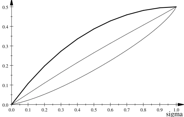
The following …gure plots the net surplus of each savvy consumer (as the middle curve),
the net surplus of each uninformed consumer (as the lower curve), and total welfare
(con-sumer surplus plus industry pro…t, plotted as the upper curve in bold). Thus, as in the
32In fact, there is an interval of pricesp which constitute this kind of “…xed price” equilibria, and the
model of price dispersion in section 2.1, each savvy consumer confers a positive search externality on other consumers. When most consumers are savvy and know the qualities
o¤ered by suppliers, suppliers compete to o¤er an e¢cient combination of price and
qual-ity, which the uninformed can usually enjoy too. When most consumers cannot discern
quality, a supplier has little incentive to o¤er high quality, and even a savvy consumer is
unlikely to secure a good product in such a market.
The model predicts that competitive …rms set a rigid price, but di¤er in their quality
which is only observed by the savvy buyers. Rational but uninformed buyers are put o¤
by a seller which o¤ers a lower price, and presume that such a seller will be cheating
on quality. A market which might …t the model is insurance, where a particular kind of insurance might be o¤ered by rival sellers at a similar price, but di¤erent sellers might have
more “exclusions” than others which only the savvy can notice and avoid.33
0.0 0.1 0.2 0.3 0.4 0.5 0.6 0.7 0.8 0.9 1.0 0.0
0.1 0.2 0.3 0.4 0.5
[image:22.595.141.457.347.548.2]sigma
Figure 3: surplus and welfare with quality dispersion
This model, and others like it, is considerably easier to analyze if the non-savvy
con-sumers are strategically naive, and do not make a connection between price and quality.
For instance, suppose that non-savvy consumers anticipate quality qe regardless of the
price asked, and so buy from the …rm with the lowest price (provided the price is below
qe). In a competitive market with many (at least four) …rms, an asymmetric equilibrium in
33Recall section 2.2, where the imposition of a price cap acted to raise average prices. One could try to
pure strategies exists of the following form: some …rms serve savvy consumers by o¤ering the e¢cient level of quality at a price which just covers cost, while other …rms serve naive
consumers by o¤ering qualityq= 0 at the price which just covers the associated cost (i.e.,
p= 0 since c(0) = 0). In such a market, the proportion of savvy types, , has no impact
on the deals o¤ered to either type of consumer, and savvy types do not protect or harm
the interests of the rest.34 We discuss a closely related model of add-on pricing in section
3.2 in more detail.
3
Hold-up
A market exhibits “hold up” when consumers are, to some extent, committed to purchasing
the product before they know the full terms of trade. For instance, if a consumer must make
a costly journey to a seller to discover its price, she might decide to buy even if the price
she …nds there was somewhat higher than she anticipated. Likewise, some consumers may
have to decide whether to purchase a product without being able to discern its quality, or
without knowing the prices of “add-on” products which later become available. We discuss
how these markets perform in situations with an indivisible good (section 3.1) and in the
more complex case with add-on pricing (section 3.2).
3.1
An indivisible product
The model of price dispersion in section 2.1 involved a market where most consumers paid
high prices when there were only a few informed consumers present. In hold-up situations,
Diamond (1971) shows how the market can break down altogether. In this section, we see
how the presence of savvy consumers can overcome or amplify this danger, depending on
the precise form of savviness.35
Suppose that a single supplier sells a product with unit cost c to a population of
consumers. Consumers di¤er in their reservation value for the item, v, where the fraction
of consumers with v p is denoted q(p). Suppose for now that all consumers know their
value v in advance. Crucially, all consumers must incur a travelling cost t > 0 to reach
34Armstrong and Chen (2009) analyze a related model where mixed strategies are used, and …nd a
symmetric equilibrium in which …rms o¤er random prices and obtain positive pro…ts, and where price is a perfect indicator of quality, i.e., if a …rm chooses a high price it will also choose high quality. However, the naivete of the uninformed consumers prevents them acting on this indicator. In this equilibrium, the fraction of savvy types does a¤ect the surplus obtained by the savvy and naive consumers.
the seller. Thus, the type-v consumer will choose to travel to the seller if v t+ ~p, if she observes (or expects to pay) price p~. Suppose a fraction of consumers (independent of
v) are savvy and know the seller’s true price in advance (but still incur the cost t if they
choose to buy), while the remaining 1 have to travel to the seller to discover its price.
These 1 ignorant consumers are rational, though, and anticipate the seller’s incentive
to set its price.
The equilibrium price is derived as followed. Suppose that p is the price that an
uninformed consumer expects to pay. If the seller actually chooses the price p, where p is
not too much bigger than thanp in the sense that p p +t, its demand is
q(p+t) + (1 )q(p +t) :
The informed travel to the seller (and buy) ifv p+t, while the uninformed travel to the
…rm ifv p +tand once at the seller they buy provided thatv p. Thus, similarly to the
model in section 2.1, the demand from the uninformed is inelastic, at least with respect
to local changes around p . Since the …rm is free to choose its price p given the price
anticipated by the uninformed consumers, an equilibrium price p is such that choosing price p=p must
maximizep p +t: ( q(p+t) + (1 )q(p +t)) (p c):
This problem has …rst-order condition
q(p +t) + (p c)q0
(p +t) = 0 : (10)
If the demand function q( ) is log-concave, this …rst-order condition has a single solution
which determines the equilibrium pricep .36
If = 1, then the equilibrium price is the price that maximizes pro…t (p c)q(p+t).
If = 0, though, so no consumers know the price in advance, no consumer chooses to
travel to the seller, and the market breaks down altogether. The seller knows that every
consumer is willing to paytmore than their anticipated pricep for the item, and so it has an incentive to set its price at least equal top +t, and there is no equilibrium price which
induces any consumer to incur the travel cost t. When some consumers are informed in
advance, though, the market opens, which is to the advantage of both consumers and the seller.
Whenq( )is log-concave, formula (10) implies that the equilibrium price is a decreasing
function of . Therefore, all consumers—savvy and uninformed—bene…t when rises.
Since the equilibrium pricep is above the monopoly price that maximizes (p c)q(p+t),
and this pro…t(p c)q(p+t)is single-peaked inp, it follows that the …rm too is better o¤
when is larger. Thus, this market provides an example where the search externality is
present, and where boosting the fraction of savvy types bene…ts all parties.37 (By contrast,
in section 2.1 industry pro…ts were decreasing in the fraction of informed consumers.)
Contrasting e¤ects are seen if some consumers know their valuevin advance rather than
the price. Suppose that no consumer knows the price in advance, so the danger of hold-up
is present. However, a fraction of consumers are savvy in the sense that they know their
valuev in advance, while the remaining1 consumers only discover their valuation once they travel to the seller and inspect the product. (These uninformed consumers view the
distribution of uncertain values to be governed by the functionq.)
An uninformed consumer who expects to pay pricep will travel to the seller if expected
surplus is greater than their travel cost, i.e., ift s(p ), where
s(p)
Z 1
p
q(~p)dp ;~ (11)
is net consumer surplus (the “area under the demand curve”) with price p. Informed
consumers, by contrast, will travel to the seller if t v p . Provided thats(p ) t, the
seller’s demand when it chooses price p p +t is
q(p +t) + (1 )q(p) ;
since all uninformed consumers travel to the seller, and they will buy if they discover that
v p. Thus, now the informed consumers have locally inelastic demand. An equilibrium price p is such that choosingp=p must
maximizep p +t: ( q(p +t) + (1 )q(p)) (p c);
which has …rst-order condition
q(p +t) + (1 )q(p ) + (1 )(p c)q0
(p ) = 0 : (12)
37As in section 2.2, therefore, pro…ts can be increased if a price cap is imposed, albeit for a very di¤erent
Following similar arguments to those used when some consumers knew the price in ad-vance, whenqis log-concave, the …rst-order condition for this problem uniquely determines
the candidate equilibrium price, but now this price p increases with . When = 0, the candidate price is the monopoly price pM which maximizes (p c)q(p), while when = 1
the candidate price is such that q(p +t) = 0. If the requirement s(p ) t fails, the
un-informed have no incentive to participate, and when this happens the market shuts down.
When the travel cost t is so large that t > s(pM), the uninformed will not travel to the
…rm even in the most favorable case when = 0. However, if t < s(pM), then the market
opens if is su¢ciently small (and fails when is close enough to 1).
In the range of where the market opens, the equilibrium price increases with , and all consumers as well as the …rm are worse o¤ with larger . When the market is open,
savvy consumers obtain a higher surplus than the uninformed, since a consumer would
prefer to know her valuation before deciding to travel to the …rm. (Expected surplus of
a savvy consumer is VS = s(p +t), while expected surplus of an uninformed consumer
is VN = s(p ) t, which is smaller.) Since demand from the uninformed, q(p ), is higher
than from the informed, q(p +t), the …rm obtains more pro…t from the non-savvy, and
N > S.
To illustrate, in the linear demand example where q(p) = 1 p and c = 0, the price which solves (12) is
p = 1 t
2 : (13)
At this price, the requirement that s(p ) t is never satis…ed when t s(pM) = 1 8, in
which case the market shuts down. Ift < 1
8, however, the market is open if the fraction of
informed consumers is su¢ciently small.38 In this example, aggregate consumer surplus
V and pro…ts both decrease with , and hence welfare does too.
Using the terminology of section 1, in formal terms this market exhibits a ripo¤ ex-ternality.39 Uninformed consumers may be willing to invest in travelling to the seller to
discover their valuation, for the chance they like the product, and this helps the market
remain open.40 However, despite the fact that
N( )> S( ), it is perhaps misleading to
38The precise condition is that 1 2p2t
1 p2t t.
39Using similar analysis to that in section 2.2 one could investigate the equilibrium proportion of savvy
consumers, when a consumer can choose to become informed of her valuationex ante by incurring a cost . Because a ripo¤ externality operates in this market, we expect that too many consumers choose to become informed in equilibrium.
price-say that the uninformed consumers are being “ripped o¤”. Unlike the market described in the next section, the seller here is not engaging in any tactic which aims to exploit this
group of consumers.
3.2
Add-on pricing
Hold-up can also occur when a seller supplies an “add-on” product once a consumer has
purchased the initial “core” product. Familiar examples of this phenomenon include: the
minibar inside a hotel room; toner cartridges once one has purchased a printer; after-sales care for your new car; an extended warranty for your new television; the ability to obtain
a casual overdraft from your bank without prior agreement, or the ability to have your
luggage stored in the aircraft’s hold in the event it is deemed slightly too large for the
cabin.
In some of these examples, it may be that the …rm does not choose its add-on price
until the customer has purchased the core product, in which case the …rm is tempted to
set monopoly prices for these services. In other cases, though, the …rm chooses both prices
at the same time, and the issue is not one of lack of commitment. Rather, the problem
is that some consumers either do not observe the …rm’s choice of add-on price, or can observe it but do not think it will apply to them. In this section we explore these cases
where …rms choose both prices simultaneously, but some consumers cannot, or do not,
take adequate notice of the add-on price. Three variants are discussed: the …rst where
non-savvy consumers are rational, but cannot see or interpret the add-on price; a second
where naive consumers do not foresee their demand for the add-on service, and a third
where naive consumers can be tricked into paying for add-ons they don’t want. Perhaps
surprisingly, these apparently small changes in model assumptions generate all three of the
market scenarios listed in section 1.
Rational but uninformed consumers: Here we assume that some consumers have prohibitive costs for reading and/or understanding the “small-print” in the contract to discover terms
for add-ons, although they do care about these terms. (More generally, the following
discussion is isomorphic to a model in which …rms choose the quality of their product, and
only a fraction of consumers are able to discern quality directly.)
A single seller supplies a core product, for which consumers have heterogeneous value
X. The price of this product is denotedP and its unit cost isC. The fraction of consumers
with X P is denoted Q(P). Once a consumer has purchased this core product, an
add-on product becomes available. The price of this product is p and its unit cost is c. All
consumers have the same add-on demand, and with price p a consumer will consume q(p)
units of the add-on service.41 Write (p) (p c)q(p) for the add-on pro…t with price
p, and pM for the price which maximizes this pro…t. The expected net surplus from the
option of being able to buy the add-on at pricep iss(p)in (11). Thus, if a consumer with
valuation X anticipates (or observes) the add-on price p~, she will buy the core product if
X+s(~p) P : (14)
If she does buy the core product, she will go on to generate add-on pro…t (p), wherep is
the …rm’s true add-on price.
Suppose a fraction of consumers observe the …rm’s true add-on price, while the
remaining 1 do not. If the uninformed expect to pay add-on price p , the …rm’s
expected pro…t from the two groups of consumers is
( Q(P s(p)) + (1 )Q(P s(p ))) (P C+ (p)) : (15)
Let(P ; p ) denote the equilibrium pair of prices. If we assume passive conjectures,
unin-formed consumers anticipate the add-on price p even if they observe an unexpected core
price P 6=P .42 For these prices to constitute an equilibrium, choosing (P; p) = (P ; p )
maximizes (over any pair of prices P and p) the expression (15). The two …rst-order conditions for this problem are
Q(P s(p )) +Q0
(P s(p ))fP C+ (p )g= 0 ;
Q(P s(p )) 0
(p ) + q(p )Q0
(P s(p ))fP C+ (p )g= 0 :
41This elastic demand for the add-on service could be generated if each consumer has a unit demand
for the add-on, with incremental valuation v, and the probability that v is above p is q(p). With this interpretation, the realization ofv is not known to the consumer (even a savvy consumer) until after she buys the core product, and is independently distributed fromX.
42When some consumers see one dimension of a seller’s choice but not another, this raises the issue of
Eliminating terms inP reveals that the add-on price satis…es 0
(p ) = q(p ), or
(1 )q(p ) + (p c)q0
(p ) = 0 ; (16)
which has a similar form to the earlier expression (10). Thus, when = 1, the add-on
price is at its e¢cient level p = c, while when = 0 the add-on price is the monopoly
price pM which maximizes (p). More generally, when add-on demand q( ) is log-concave,
formula (16) implies that the add-on price is a decreasing function of . For example, when
q(p) = 1 p and c= 0, the add-on price is p = 1 2 .
It is straightforward to show that consumers and the …rm are worse-o¤ when the
equi-librium add-on price is higher, i.e., when is smaller.43 Thus, this market exhibits search
externalities of the strong kind where all parties are better o¤ when the fraction of in-formed consumers rises. In this it is like the hold-up model with an indivisible product
discussed above.
This discussion implicitly assumed that the seller had to o¤er the same add-on terms
to all its customers, which seems a reasonable assumption in most contexts. (It is hard to
imagine a hotel supplying rooms with di¤erent minibar prices, for instance.) If feasible, though, the seller has an incentive to set di¤erent add-on terms: an e¢cient price p = c
aimed at the savvy, and a monopolistic price p= pM aimed at the savvy. (The
non-savvy might accidently choose the e¢cient contract, but this probability could be reduced
if the seller somehow o¤ered the monopolistic contract, together with a “hard-to-…nd”
e¢cient contract which only the savvy could locate.) The fact that the seller o¤ers the
same deal to all consumers immediately implies that VS =VN and S = N.
This framework with rational but uninformed consumers is hard to extend to
compet-itive environments, except in the extreme cases where = 0 or = 1.44 The model with
quality dispersion in section 2.4 has this ‡avour, and could presumably be re-interpreted as a model of add-on pricing after suitable adjustments. Much easier to analyze, and arguably
43To see this, writeY =P s(p)for the “total price” for the core product. Then consumers are better o¤ whenY is smaller. For given equilibrium add-on pricep , the …rm chooses the core pricePto maximize Q(P s(p ))(P C+ (p )), i.e., it chooses the total priceY to maximizeQ(Y)(Y C+w(p )), where w(p) s(p) + (p)is total add-on surplus with add-on pricep. The functionw(p)is decreasing forp c. SinceY maximizesQ(Y)(Y C+w), a higher w(i.e., a lower p ) is like the monopolist having a lower cost, which induces a lowerY and higher optimal pro…ts.
44Ellison (2005) presents a Hotelling-style duopoly model of add-on pricing. He analyzes two games: one
where the two …rms reveal both of their pricesex ante and another where neither …rm reveals its add-on price until consumers buy the core product. Using the current notation, these two cases correspond to