Flow through the Strait of Dover

INTERNAL DOCUMENT

FLOW THROUGH THE STRAIT OF DOVER

D. PRANDLE

lOS INTERNAL DOCUMENT 148

fThis document should not be cited in a published bibliography, and is supplied for the use of the recipient only].

INSTITUTE OF • CEAIMOGRAPHIC SCIENCES

%

INSTITUTE OF OCEANOGRAPHIC SCIENCES

Worm ley, Godalming, Surrey, GU8 BUB.

(042-879-4141)

(Director: Dr. A . S. Laughton)

Bidston Observatory,

Birkenhead,

Merseyside, L43 7RA.

(051-652-2396)

(Assistant Director: Dr. D. E. Cartwright)

Crossway,

Taunton,

Somerset, T A 1 2DW.

(0823-86211)

FLOW THROUGH THE STRAIT OF DOVER

D. PRANDLE

lOS INTERNAL DOCUMENT 148

ABSTRACT

This report has been compiled for the use of engineers involved in the design of bridge/tunnel crossings of the Dover Strait. Detailed information is provided on elevations, velocities and

1. INTRODUCTION

Recently there has been renewed interest in the construction of a rail or road

connection across the Dover Strait. Schemes under consideration include a proposed

bridge and tunnel link with the bridge sections extending many kilometres into the

Strait from both ends. Clearly schemes of this sort, which involve crossing the

Strait as opposed to simply tunnelling underneath, require a detailed knowledge of

local flow conditions. The present report aims to provide a substantial part of

this information on flow conditions.

This region is one of the world's busiest navigation routes and as such has

been studied extensively for many years. The shipping density and high currents

combine to make off-shore measurements difficult and hazardous. Nevertheless, in

recent years a number of oceanographic recordings have been made throughout this

region. Inter-comparison of these recordings has proven their accuracy and

reliability. Additionally, use is made here of a fine-grid (2.5 km) numerical

model of the tidal propagation in the region to supplement observational data and

to provide detailed spatial coverage.

A major part of this report deals with tidal propagation and information is

provided for elevations, currents and net flows through the Strait. Meteorological

influences, in particular the effect of wind-forcing, are also examined in some

detail under the heading of "surges".

Wherever practical, essential information is listed here, otherwise references

to basic sources are given. This report does not include information on (a) the

wind-wave climate, (b) internal-waves or (c) sedimentation. The combination of

high currents in relatively shallow depths promote rapid vertical mixing and )

probably preclude the propagation of interval-waves through this region.

2. OBSERVATIONAL DATA

The Dover Strait connects the southern North Sea with the English Channel

subject to occasional high storm activity. The narrowest section is about 34 kms

wide with depths of up to 50 m (figure 2).

2.1 Currents

Doodson (1930) analysed currents observed at the Varne Light-vessel (50°56'N,

1°17'E) over a two year period from 1922 to 1924. Recordings were taken 3 times

daily at six depths, the tidal constituents derived from these recordings are

discussed in section 4.

From 1920 to 1924, Carruthers (1925, 1927) used drift bottles to study the

eastwards drift from the western end of the English Channel along the continental

coast as far as the German Bight and beyond. These drift patterns established by

Carruthers have been verified and quantified further by recent studies of the

movement of Caesium released from the French nuclear plant at Cherbourg (Kautsky

1976). Carruthers (1928, 1935) also used a long series (1926 to 1932) of current

meter recordings from the Varne to study the residual drift through the Dover

Strait and, in particular, the relationship between this drift and the prevailing

wind conditions.

Van Veen (1938) carried out an exhaustive series of current meter recordings

throughout the Dover Strait region over the period 1934 to 1936. In total, he

measured 300 profiles at 31 locations and in 1936 a further 392 profiles from a

single location approximately 5 miles from Dover. From these measurements, he

arrived at a parabolic representation for current profile in this region with

V » where V ^ ) the velocity at height X above the bed is

related to the surface velocity \/^ , D is the water depth and 0.0%,

Van Veen derived tidal constants for 7 constituents and made estimates of average

flood and ebb flow through the Strait and thereby the net residual flow.

In more recent times, flow measurements through the Dover Strait have been

made by using cross-channel submarine telephone cables. The flow of a conducting

earth's field, induces a potential difference proportional to the rate of flow.

Bowden (1956) recorded this potential difference, using the telephone cable

running from St. Margaret's Bay to Sangatte, over a 15 month period in 1953 and

1954. By comparing the voltage recordings with the tidal flow as predicted by

Van Veen (1938) a calibration coefficient relating voltage to flow was deduced.

Using this calibration coefficient, Bowden deduced flow magnitudes associated

with eight tidal constituents. In addition, by examining the non-tidal component

of the cable voltage he deduced a relationship between daily-mean values of flow,

surface gradient and wind speed.

Cartwright (1961) and Cartwright and Crease (1963) also used cross-channel

cable measurements to deduce the average sea-surface gradient between Dover and

Dunkirk. Part of this study involved direct measurements of current profiles at

six positions across the Strait over a five day period.

In 1973 the first deployment of automatic self-recording current meters was

made in the Dover Strait. Recordings at three locations were obtained for periods

of up to 49 days (Howarth and Loch 1977). The recordings formed part of an

international oceanographic exercise in the southern North Sea referred to as

JONSDAP '73. During this same exercise, simultaneous current measurements were

made at four locations across the Strait over a period of 25 hours. These

recordings are described by Prandle and Harrison (1975b). This paper also provides

details of cable measurements recorded over a five-month period in 1973.

2.2 Elevations, salinity, temperature and meteorological data

A number of ports are located within the Dover Strait region (figure 1) and

consequently shore-based tidal elevation data are plentiful. Table 1 shows the

values of eight major constituents from ten ports. In addition, this table shows

data from an off-shore tide gauge, TI, deployed for 46 days in 1973.

Long terra monthly-mean values of temperature and salinity of the sea water

available from Light-vessels and can be obtained from the Marine Information

Advisory Service (M.I.A.S.) of I.O.S. Meteorological data are also available

from these Light-vessels as well as from land-based recording stations. Wind

data from Lympne, near Dover, have been used in studies of wind driven currents

in this region (e.g. Bowden 1956). However, data recorded at sea are often more

representative and Prandle (1978b) made use of data from the Dutch Light-vessel,

Noord Hinder (51°39'N, 2°34'E). An alternative source for wind data may be

obtained by using gradients of atmospheric pressure, by this means Schott (1970)

calculated monthly mean winds for this region over the period 1950 to 1967.

3. NUMERICAL MODEL

The outer model of the southern North Sea extends northwards to latitude 53°20'

and westwards to the Greenwich meridian (figure 1). The model is two-dimensional

with velocities vertically averaged, the grid follows lines of latitude and

longitude with spacings of 10*of longitude and 6|-^of latitude, i.e. approximate

12 km. In the Dover Strait region, between latitudes 50°46y' and 51°20', this

grid is sub-divided by a factor of five resulting in a grid size approximately

2.5 km square. A comprehensive description of the numerical finite difference

scheme employed is given by Prandle (1974). In the present application the use

of a smaller grid size with an explicit finite difference scheme required the

time-step to be reduced to 1 minute. The coupling between the fine and coarse

grids was fully dynamic and hence the boundaries of the model were at the

positions stated previously.

The dynamical equations used are :

. . A

+ u^_u_+ + Q + q c o u ( u + v ) — r w — 0 (1)

+

^ z + ^ j u C z - t t i ) ] Jl ^ ^ V ( x + 0 Q )

8 b

3x

Ax

where U , V are depth mean velocities along the ic and ^ axes respectively,

orthogonal axes positive to the east and to the north,

A x grid length in the x. direction,

%. elevation of the water surface above a horizontal datum,

0 depth of the bed below the same datum,

p density of sea water,

Co a friction coefficient, constant throughout the model,

fl Coriolis parameter,

t time,

^ gravitational acceleration.

For clarity the terms representing the influence of wind forcing and atmospheric

pressure have been omitted from (l) and (2).

Model results cited in later sections were, in most instances, taken from a

simulation of tides over a 15-day period, i.e. a complete spring-neap-spring cycle.

4.' TIDES

4.1 Elevations

In the terminology used for tidal predictions, Dover is classified as a

shallow-water port. This implies that non-linear interactions are important in this

vicinity and, as a result, accurate tidal predictions by the "harmonic method"

requires the use of 114 tidal constituents. The predominant constituent is with

an amplitude of 2.23 m followed by with an amplitude of 0.71m and with

ampli-tude 0.41 m. Interest here will be restricted to these three major constituents

together with the diurnal constituents 0^ and and the higher harmonics M^, MS^

exceptions of (0*10 m), Lg (0.14 m) and (0.20 m). The amplitude and phase

of these eight constituents were previously shown in table 1 for 10 ports in the

region and for one off-shore tide gauge, TI.

Prandle (1980) produced co-tidal charts for the southern North Sea and Dover

Strait region for these eight constituents. The charts were constructed on the

basis of all available tidal data (both tide gauge and current meter data)

together with tidal distributions obtained from a numerical model of the region.

For most purposes, these charts provide sufficient information on the propagation

of tidal elevations through the Dover Strait. Similar co-tidal charts for the

English Channel have been produced by Chabert D'Hieres and Le Provost (1978).

Figures 3(a) and 3(b) show a comparison of model and observed results for the

amplitude and phase of the constituent, likewise figures 4(a) and 4(b) show

similar comparisons for S^. The results shown by Prandle (1980) should be used

for data extraction, these latter figures are only included to indicate the

accuracy of model results in this region. The results for show that the phase

values in the model are in almost precise agreement with observation but that

model amplitudes are about 10% larger than observations on the British coast and

about 20% larger on the Continental coast.. The comparisons for S^ show that the

phase in the model lags behind observed values by about 10° and the amplitude in

the model is about 5% smaller than observed.

4.2 Currents

Tables 2(a) and 2(b) summarise the observed current data described in section

2.1. These data provide a good spatial representation of tidal currents in the

Strait and, allowing for localised variability, there is good agreement between

observations for all except the smallest constituents.

Component parts of figures 3 and 4 show model results for current ellipse

properties for the constituents and S^ respectively. Part (c) shows the major

direction of the major axis JL and (f) the eccentricity E. These model results

show the spatial variability of the tidal components and may be compared with the

distributions for A, G and oi. shown by Sager (1968). While Sager's results are

based on observed flow at the time of spring tide, there is close agreement between

these results and the computed values shown in figures 3 and 4.

Observed values for cL and E are indicated in figures 3(e), 3(f), 4(e) and

4(f) for ready comparison with model results. The eccentricity E denotes the ratio

between minor and major axes of the current ellipse and a sign convention is

appended to indicate direction of rotation (positive for anti-clockwise rotation).

All four diagrams indicate close agreement between model results and observations.

Figures 5(a) and 5(b) show, for M2 and $2, a comparison of observed and model

results for A and G across a section of the channel between Dover (St. Margaret's

Bay) and Sangatte. This section corresponds to the location of Cartwright's (1961)

measurements and follows the line of the cross-channel telephone cables (figure 2).

The observations from TQ, TO and TK lie a few kilometres north-east of this line

and hence the phases at these positions should show some small lag relative to the

other values. For M2, the model values for A are about 18% larger than

observat-ions and the model phase leads by almost 30°. For S2, the model values for A are

in almost exact agreement with observations and the model phase leads by about

7°. Comparing these results with those for elevations described in the previous

section (4.1), we note that for M2, the larger amplitude in the model currents

accompanies the larger range of elevation in the model. Whereas the 30° phase

lead in the currents contrasts with the precise agreement in the elevation phases.

For S2, the exact agreement in current amplitudes differs only slightly from the

5% smaller amplitudes found in the model elevations while the 10° phase lag in

model elevations is converted to a 7° phase lead in model currents.

In a more usual modelling simulation where the tidal energy propagates in a

friction in the direction from which the energy is propagating. This would normally

decrease tidal amplitudes and delay tidal phases and some suitable compromise

between the agreement for both elevations and currents could be achieved. However,

in the Dover Strait tidal energy propagates from both the English Channel and the

North Sea and the observed conditions may be seen as a vector addition of the two

tidal systems. Adjustment of the model under these conditions is clearly more

complex. In addition, it is likely that tidal conditions in the Strait might be

sensitive to small relative changes in boundary conditions specified along the

open-boundaries of the southern North Sea model (figure 1).

This latter point may be readily understood by noting, from figure 3(d) that

the current phase along the Strait changes by 30° in as little as about 10 kms and

hence only a slight modification to the spatial pattern is required to account for

the discrepancy between model results and observations. An additional point of

interest shown by both figures 3(d), 4(d), 5(a) and 5(b) is the large phase •

variation across the channel with a 'boundary' layer at each side showing phase

leads of up to 60° relative to the central section. Van Veen (1938) observed

similar effects in the boundary regions. This 'early reversal' at the boundaries

is commonly experienced in estuaries; it is attributed to bed-friction and in

mid-channel a related phase difference is generally found between flow at the bed and

at the surface. In the model, the phase of the current in this region is almost

directly related to the bed friction term and hence reflects the current phase at

the bed. The observed currents generally reflect depth-averaged conditions and no

clear mention has been made of significant phase changes through depth in these

observations. However, in view of the difficulties of measuring currents very

close to the bed in this region,it i6 possible that a significant phase advance

exists which could explain the difference between model and observed results.

The complexity of the tidal propagation can be seen from the relationship

in Table 1 with the current data from Table 2(a), we find for the semi-diurnal

constituents, that the phase of the elevation leads the current phase by about 30°,

In an estuarine system we normally expect this phase difference to vary between 0°

for a progressive wave and -90° for a standing wave. The present phase difference,

= 30°, indicates that there is a net propagation of tidal energy into the North

Sea (i.e. c o s Y •> O) and the unusual phase relationship may be attributed to the

vector addition noted earlier. (The complex results of such vector addition may

be understood by adding two arbitrary wave components and then adjusting the ratio

of current to elevation amplitude in one component). For the diurnal constituents

the phase of the elevation leads the current by an angle in the range 90° to 270°

indicating that the tidal energy propagates out of the North Sea (i.e. cos1[/'< 0).

This latter result is confirmed by the progression of elevation phases towards the

Channel for both 0^^ and shown by Prandle (1980).

Comparing the amplitude ratios of the various data sets in Tables 1 and 2(a)

we find the ratios of S2 :M2 and N2 :^2 are almost identical between various

current meters, the cable voltage and the elevation at Dover. Similarly the

ratios of M^, and to are similar for these various data sets although

some variability arises due to the inaccuracy associated with the determination of

these constituents. By contrast the ratios of 0^ : Mg and : Mg in the elevation

data are approximately one-third of the corresponding ratios in the current meter

and cable data sets. The smaller relative values of elevation for these latter

constituents may be attributed to the close proximity of amphidromic points as

shown by Prandle (1980).

Determination of the longer period tidal constituents for the flow data is

difficult due to their small amplitudes and the need for a long recording period

to eliminate meteorological effects or other 'noise components' such as

instrumental errors. From an analysis of 10 years of cable recordings, Alcock

%

V

for Mg. The value for MS^ at the same location in the model is about 2.6 cm s"^

or, again, about 1/50 of the value for

The cross-sectional area of the Dover-Sangatte line is approximately 1.22 x 10^ 2

m . By taking a vector mean of tidal constituents at TQ, TO and TK we calculate

(a) for Mg, a velocity amplitude of 106 cm s ^ or a net flow amplitude of

6 3 —1 —1

1.29 X 10 m s and (b) for a velocity of 36 cm s with a net flow of

0.44 X 10 m s . By taking a similar vector mean of Cartwright's (1961) data

we obtain (a) for 113 cm s ^ or 1.38 x 10^ m^s ^ and (b) for S^, 38 cm s ^

6 3 —X

or 0.46 X 10 m s . For the model, corresponding values are (a) for ,

130 cm s ^ or 1.43 x 10^ m^s ^ and (b) for S^, 36 cm s ^ or 0.40 x 10^ m^s ^.

5. SURGES

All non-tidal phenomena are here summarised under the heading of "surges",

in general the concern is with meteorologically generated flows. The physics

of surge generation in this region has been described by Heaps (1967), interest

here will bo restricted to flow and elevation data within the Dover Strait.

Table 3 shows pertinent elevation data for Dover taken from the Admiralty

Tide Tables (ATT) and from a study of sea level maxima carried out by Graff (1981).

The storm levels cited correspond to the highest estimates given by Graff. Table 4

shows related flow data for the Dover Strait. Values for the and S^ tide were

taken from the numerical model, Neap tide corresponds to M2 - Sg and Spring tide to

^2 ^ ^2" additional. values shown in this table were obtained by assuming the

same proportional factors as shown for the elevation data in Table 3. Thus the

ratio HAT/ in Table 3 is assumed to apply between HAT/„ . ^ , in Table 4.

MHWS •' Spring tide

From related studies carried out elsewhere it is expected that the estimates for

flow data in Table 4 might be too large, interaction effects limit extreme flows

to a greater degree than extreme elevations. As a check on these estimates we can

recorded at Dover and corresponds to the 1 in 100 year return level. Prandle

(l975a) showed that the flow through the Dover Strait for this surge reached a

maximum of about 2.50 x 10^ m^s ^ whereas Table 4 gives a value of 2.78 x 10^ m^s~^

for the 1 in 100 year storm.

It is possible that the maximum elevation and maximum flow occurring in a

particular storm do not correspond to the same level of probability. In addition,

the geometry of the surrounding regions introduces some assymetry into the

probability distribution of positive (towards the North Channel) and negative

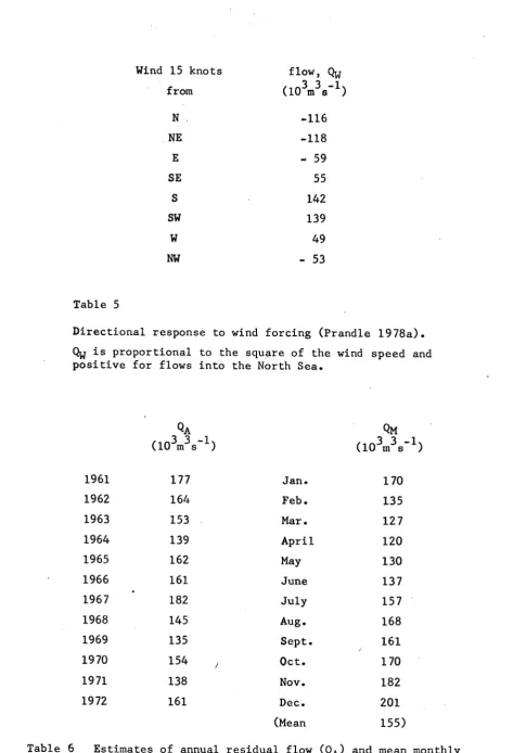
flows. Table 5 shows a relationship derived by Prandle (1978a) between wind

direction and flow through the Strait for a wind speed of 15 knots. This Table

represents an averaged response to a steady wind speed as calculated from

modelling studies. While these results were shown (Prandle 1978a) to be in good

agreement with similar results found by Bowden (1955), they should be used with

due caution. Noting that the flow is proportional to wind speed squared, the

wind speed corresponding to a particular return period can be estimated by scaling

up the values in Table 5 to account for the difference between storm flows and

maximum tidal flows as shown in Table 4. Thus the 1 in 250 year storm flow could

be obtained when a steady wind speed of 43 knots blows in a northerly direction in

combination with a spring tide. The equivalent wind velocities for the 1 in 50

and 1 in 100 year storms are 35 knots and 39 knots respectively.

In addition to the meteorologically-induced flow there is a more or less

permanent residual flow' towards the North Sea due both to the non-linearities

associated with tidal flow and to the oceanic-scale flow across the continental

shelf. The exact magnitude of this steady residual is difficult to estimate )

(Otto 1982), here it is convenient to adopt Prandle's (1978a) estimate of

123 X 10^ m^s

The fine grid model (figure l) indicates considerable variation in the

Dover-Sangatte section the residual current is towards the North Sea but in the

two intermediate zones the residual current is in the opposite direction. The

residual flow is similarly variable, although for the Dover-Sangatte section it

is always towards the North Sea with one small exception about 8 kms from Dover.

Van Veen (1938) reported similar cross-sectional variations in residual flow.

Using the above estimate for residual flow together with the relationships

between wind speed and flow shown in Table 5 Prandle (1978b) estimated

monthly-mean residual flows through the Dover Strait for the years 1949-1972. Table 6

shows part of these results listing the annual flows for the years 1961 to 1972

and the mean-monthly values averaged over the 24 year period. The monthly

References

ALCOCK, G.A. and CARTWRIGHT, D.E. 1978. An analysis of 10 years' voltage records from the Dover-Sangatte cable, pp.341-365 in, A voyage of discovery, George Deacon 70th Anniversary Volume, (ed. M. Angel). Oxford: Pergamon. 696 pp.

BOWDEN, K.F. 1956. The flow of water through the Straits of Dover related to wind and differences in sea level. Philosophical Transactions of the Royal Society of London, A, 248, 517-551.

CARRUTHERS, J.N. 1925. The water movements in the Southern North Sea. Part 1. The Surface Drift. Fishery Investigations, Ser.2, 8(2), 119 pp.

1927. Investigations upon the water movements in the English Channel. Summer, 1924. Journal of the Marine Biological Association of the U.K.

1928. The flow of water through the Straits of Dover as gauged by continuous current meter observations at the Varne Lightvessel. Part 1. Fishery Investigations, Ser.2, 11(1), 109 pp.

1935. The flow of water through the Straits of Dover. Fishery Investigations, Ser.2, 14(4), 67 pp.

CARTWRIGHT, D.E. 1961. A study of currents in the Straits of Dover. Journal of the Institute of Navigation, 14(2), 130-151.

CARTWRIGHT, D.E. and CREASE, J. 1963. A comparison of the geodetic reference levels of England and France by means of the sea surface. Proceedings of the Royal Society of London, A, 273, 558-580.

CHABERT D'HIERES, M.G. and LE PROVOST, C. 1978. Atlas des compasantes harmoniques de la maree dans la Manche. Annales Hydrographigues, Ser.6, 5-36.

DOODSON, A.T. 1930. Current observations at Horn's Rev., Varne and Smith's Knoll in the years 1922 and 1923. Journal du Conseil, 5, 22-32.

GRAFF, J. 1981. An investigation of the frequency distributions of annual sea level maxima at ports around Great Britain. Estuarine, Coastal and Shelf Science, 12, 389-449.

HEAPS, N.S. 1967. Storm Surges. Oceanography & Marine Biology, an annual review, 5, 11-47.

HOWARTH, M.J. and LOCH, S.G. 1977. Moored current meter records, southern North Sea; 6 Sept. - 28 Oct. 1973; 10S Bidston Moorings 37-43. Institute of Oceanographic Sciences, Data Report No.14, 102 pp. (Unpublished manuscript).

KAUTSKY, H. l976. The Caesium 137 content of the North Sea during the years 1969 to 1975. Deutsche Hydrographische Zeitschrift, 29(6), 217-221.

PRANDLE, D. 1974. A numerical model of the southern North Sea and River Thames.

Institute of Oceanographic Sciences, Report No.4, 24 pp. (Unpublished

manuscript).

PRANDLE, D. 1975a. Storm surges in the southern North Sea and River Thames. Proceedings of the Royal Society of London, A, 344, 509-539.

PRANDLE, D. and HARRISON, A.J. 1975b. Relating the potential difference measured on a submarine cable to the flow of water through the Strait of Dover.

Deutsche Hydrographische Zeitschrift, 28, 207-226.

PRANDLE, D. 1978a. Residual flows and elevations in the southern North Sea. Proceedings of the Royal Society of London, A, 359, 189-228.

PRANDLE, D. 1978b, Monthly mean residual flows through the Dover Strait, 1949-1972. Journal of the Marine Biological Association of the U.K., 58, 965-973.

PRANDLE, D. 1980. Co-tidal charts for the southern North Sea. Deutsche Hydrographische Zeitschrift, 33, 68-81.

SAGER, G. 1968. Tidal streams in the Straits of Dover. Seeverkehr 11, 458-460.

SCHOTT, F. 1970. Monthly mean winds over the sea areas around Britain during 1950-1967. Charlottelund Slot, Denmark : International Council for the Exploration of the Sea, Hydrographic Service. 17 pp.

SMED, J. 1970. Monthly means of surface temperature and salinity for areas of the North Sea and the north-eastern North Atlantic. Charlottelund Slot, Denmark. International Council for the Exploration of the Sea, Hydrographic Service.

List of figures

1. Schematic representation of the southern North Sea and Dover Strait.

2. Dover Strait : depth contours, observational locations and submarine cable

alignment.

3. Propagation of the M2 tide through the Dover Strait.

Contours indicate model results and point measurements indicate observed values (units cgs)

(a) elevation amplitude;

(b) elevation phase (relative to the lunar transit at Greenwich); (c) amplitude of the major axis of the current ellipse, A ;

(d) phase of the maximum current, 6 ;

(e) direction of the major axis, aL , measured clockwise from north; (f) eccentricity, E.

E is defined as the ratio of the minor axis : major axis, in addition E is positive for an anticlockwise rotating ellipse and negative for clockwise rotation.

4. Propagation of the S2 tide through the Dover Strait.

Legend as for Figure 3.

5. Comparison of observed and model results for currents across the

Dover-Sangatte section.

A - major axis; G current phase.

model, Cartwright's (1961) measurements;

• TO, TQ and TK.

List of Tables

1. Tidal Elevations.

Amplitude (cm) and phase (g) of major tidal constituents.

Sources : ICOT '63 Institute of Coastal Oceanography and Tides ('63 indicates year of observation).

ATT Admiralty Tide Tables.

IHB International Hydrographic

Bureau-EPSHOM Establissement Principal du Service Hydrographique et

Oceanographique de la Marine. /

Data length; Y - year, D - day.

2. (a) Current Observations.

Amplitude of the major axis of the ellipse (cm s ^). Phase of the maximum current.

Cable data in mV.

16

(b) Additional current ellipse data.

Direction of the major axis measured clockwise from north. Ellipticity, negative indicates clockwise rotation.

3. Elevation data for Dover.

Sources : Tidal data - ATT, storm levels - Graff (1981). Data in metres above O.D.N., chart datum = -3.67 O.D.N.

4. Average velocities and total flow through the Dover Strait

(Dover-Sangatte section).

5. Directional response to wind forcing (Prandle 1978a).

QW is proportional to the square of the wind speed and positive for flows into the North Sea.

6. Estimates of annual residual flows (Q ) and mean monthly values (Q ),

LOCATION

LAT N

LONG

E SOURCE

DATA

LENGTH °1

%2 ^2 =2 "4 MS, 4 ^6

Rarasgate 5l°20 1°25 ICOT '63 1 Y 9,182° 7,12° 35,318° 186,339° 56,30° 13,241° 8,287° 4,125°

Deal 51°13 1°25 _ATT 7,175° 6,20° _{207,336° 63,27°}

Dover 51°07 1°19 10S '75 1 Y 6,172° 6,46° 41,309° 223,332° 71,23° 27,220° 17,273° 7,104°

Folkestone 51°05 1°12 ATT 2,241° 5,55° 245,332° 79,32°

Hastings 50°51 0°35 IHB 30 D 2,223° 8,95° 44,294° 247,323° 89,17° 22,228° 15,283° 4,173°

Ostend 51°14 2°55 ICOT '43 1 Y 8,174° 4,346° 29,339° 176,5° 52,58° 9,337° 7,37° 7,300°

Nieuport 51°09 2°43 ICOT '43 1 Y 10,174° 5,354° 32,336° 186,0° 54,52° 13,310° 8,8° 5,268°

Dunkirk 51°03 2°22 ICOT '58 1 Y 7,157° 4,9° 36,330° 211,353° 63,46° 15,279° 9,337° 3,214°

Calais 50°58 1°51 ICOT '41 1 Y 4,147° 1,62° 43,320° 238,341° 76,33° 22,241° 15,295° 5,125°

Boulogne 50°44 1°35 EPSHOM 1 Y 4,77° 18,135° 52,310° 293,331° 96,21° 33,222° 22,275° 6,90°

TI 51°09 1°47 ICOT '73 46 D 10,162° 6,26° _{35,324 206,345° 66,35° 17,253° 14,297° 3,157°}

Table 1. Tidal Elevations.

Amplitude (cm) and phase (relative to the moon's transit at Greenwich) of major tidal constituents. Sources: ICOT '63; Institute of Coastal Oceanography and Tides ('63 indicates year of observation).

ATT : Admiralty tide tables.

IHB : International Hydrographic Bureau.

EPSHOM ; Etablissement Principal du Service Hydrographique et Oceanographique de la Marine.

LAT LONG DATA

Ol • Kl _%2

SOURCE N E LENGTH Ol • Kl %2 ^2 32 %4 M S ^ ^6

Doodson (1930) 1922 50°56 1°17 l Y 9,217° 11,84° 72,0° 23,56° 5,72°

1 9 2 3 l Y 6,204° 6,21° 78,348° 26,27° 1,185°

Van Veen (1938) 51°04 1°25 16D 13,31° 10,177° 109,7° 26,60° 10,286°

TK J'73 51°05 1°47 46D 11,46° 11,193° 19,357° 105,5° 36,54° 13,276° 11,319° 2,179°

TQ J'73 51°09 1°31 44D 12,52° 12,181° 22,0° 106,8° 33,53° 13,286° 8,176° 3,204°

TO J'73 51°04 1°35 32D 11,56° 11,201° 20,353° 108,11° 38,57° 12,274° 9,315° 2,168°

C Cartwright 1961 51°07 1°26 2D 8,335° 5,199° 16,333° 103,354° 35,45° 12,274° 8,323° 5,220°

B " 51°05 1°30 2D 11,4° 8,228° 20,353° 121,14° 41,65° 22,293° 14,342° 1,110°

A " 51°04 1°33 2D 14,12° 8,236° 18,352° 110,13° 37,64° 22,268° 14,317° 2,358°

A " 51°02 1°35 2D 13,9° 8,233° 17,349° 107,10° 36,61° 19,284° 12,333° 1,290°

B' " 51°0 1°38 2D 12,345° 7,209° 20,341° 124,2° 42,53° 20,260° 12,309° 1,149°

C " 50® 59 1®41 _2D 9,0° 5,224° 18,331° 119,352° 38,43° 16,257° 10,306° 6 , 2 0 4 °

Cable Data, Prandle & Harrison (1975b) 128D 81,41° _{60,199° 132,343° 7 2 0 , 1 ° 2 5 9 , 5 2 ° 8 0 , 2 8 5 ° 5 8 , 3 3 3 ° 12,190°}

- 1 Table 2(a) Current Observations.

Amplitude of the major axis of the current ellipse in cm s"

Phase of the maximum current (for velocities approximately NE except as stated in table (b) ). Cable data in mV.

K, Nr M, MS, M,

Doodson 1922

1923 TK TQ TO 54",-.02 53°,-.02 47",-.05 50°,-07 41",-.01 53°,-.13

54",-.00 57",-.02

40°,.02 57°,.03 53°,.04 42°,.02 51",-.04 33°,-.16 34°,-.15 54°,.06 43°,-.08 51°,.02

36" i°,-.20 14

3 3 ° ,

-55°,.07 42°,- .09 51°,.01 50°,.10 45°,.06 56°,.20 272",-.09 23°,-.08 50°,.11 55°,.23 45°,.18

329",-.38 38°,-.18

61°,.53

Table 2(b) Additional current ellipse data.

Mean Low Water Springs (MLWS)

Mean Low Water Neaps (MLWN)

Mean Water Level (MWL)

Mean High Water Neaps (MHWN)

Mean High Water Springs (MHWS)

Highest Astronomical Tide (HAT) 1 in 50 year Storm Level

1 in 100 year Storm Level 1 in 250 year Storm Level

- 2.87 - 1.67 .03 1.63 3.03 3.63 4.37 4.58 4.89

Table 3 Elevation data for Dover.

Sources, tidal data ATT, storm levels, Graff (1981). Data in metres above ODN; chart datum = -3.67 ODN.

Mg tide Sg tide Neap tide Spring tide HAT

1 in 50 year Storm 1 in 100 year Storm 1 in 250 year Storm

Average velocities (m s ^)

1.30 .36 0.94

1.66

1.43 0.40 1.03 1.83

2.20

Table 4 Average velocities and total flow through the Dover

Table

Wind 15 knots flow, %

from ( l O ^ m ^ s' b

N . -116

NE -118

E - 59

SE 55

S 142

sw 139

w 49

NW - 53

Table 5

Directional response to wind forcing (Prandle 1978a).

Qy is proportional to the square of the wind speed

positive for flows into the North Sea.

and

3 ' ^ - 1 (10 m s )

Qm

(10\^s' b

1961 177 Jan. 170

1962 164 Feb. 135

1963 153 Mar. 127

1964 139 April 120

1965 162 May 130

1966 161 June 137

1967 182 July 157

1968 145 Aug. 168

1969 135 Sept. 161

1970 154 , Oct. 170

1971 138 Nov. 182

1972 161 Dec.

(Mean

201 155)

6 Estimates of annual

values (Qj^) (Prandl

residual flow (Q^) e 1978b).

LOWESTOFT

UMUIDEN

HOEK VAN HOLLAND

WALTON

SOUTHEND

RAMSGATE

OSTENO DEAL

DOVER

FOLKESTONE A NIEUPORT

DUNKIRK

HASTINGS C A L A I S

& BOULOGNE

DIEPPE

5 I * N

-5 0 » -5 0 ' N

ST. MARGARET

DOVEff?,

^SANGATTE

vorn»

SUBMARINE CABLE CONTOUR DEPTHS IN METRES • VELOCITY MEASUREMENTS wk. OFF-SHORE TIDE GAUGE

f 2 0 ' E l»30'E

51° 2 0 '

&l°00'

i°oo' 2 ° 0 0 ' 3 ° 0 0 '

( a )

. 2 4 0 -• 206

\

y ( a )

. 2 4 0 -• 206

\

^

280"'

3 0 0 J

5 I ° 2 0 ' 1*00' 2 ° 0 6 '

51 " 0 0 '

* s W

( b )

3 3 9 1 ^ \ 336*4 345°

3 3 ^ \ A

\

0 " w/ l

3 2 3 % ^

330*

> ^ 4 1 "

Jzzx"

( c )

\ 120

^

/

\

i

( d ) P N

) /

1 5 °

-( d )

" / \ ^

^ p 7 (

^ 3 3 0 °

3 l 5 t ^

( f )

X.°=o w

y ? " ' . V / \ 0 0 7 ^

J /.&//

. ( - 0 1 5 \ X

3. Propagation of the M2 tide through the Dover Strait.

Contours Indicate model results and point measurements indicate, observed values (units cgs)

( a ) elevation amplitude; (d) p h a s e of the m a x i m u m current, G ;

(b) elevation phase (relative to the lunar transit at Greenwich); (e) direction of the major axis, 4^ , measured (c) amplitude of the major axis of the current ellipse, A ; (f) eccentricity, E.

' • " O ' 5 , - 2 0 ' ro(/ 2°0(/

s i ' o o '

( b ) _{2 7 ° 4 \}

z ^ l / \ s A

! M \ V

^ \ \ \

\

"""^4^

JA\'

( 0

/ ,/

20

(

\iA

( d )

330° 6

3 0 0 ° ^ — r i / L / X ^

( e )

fc

y\

*

<

J ,60

6

V x"

)

•

( f )

r //

* / )

^ % - 0 09 / ( V X X \ y ^ O I 0 0 7 >

^ 0 3 X /

^ 0 2

; \

1 \

X I

- 0 1 7 \ ^ y X

4. Propagation of the 82 tide through the Dover Strait.

15

1 0

A

0 5

1 5 r

1 0

A

0 5

Dover TQ TO TK Sangatte Dover TQ TO TK Sangatte

30

Q

- 3 0

#

6 0

e

30

( a ) M z ( b ) S i

5. Comparison of observed and model results for currents across the Dover-Sangatte section.

k - major axis; 8 current phase.