Munich Personal RePEc Archive
Electoral Systems and Corruption: the
Effect of the Proportionality Degree
Alfano, Maria Rosaria and Baraldi, Anna Laura and
Papagni, Erasmo
Department of Economics - Second University of Naples,
Department of Economics - Second University of Naples,
Department of Economics - Second University of Naples
3 January 2014
Online at
https://mpra.ub.uni-muenchen.de/53138/
1
Electoral Systems and Corruption:
the Effect of the Proportionality Degree
Maria Rosaria Alfano
Dipartimento di Economia, Seconda Università di Napoli, C.so Gran Priorato di Malta – 81043 Capua (Italy). [email protected]
Anna Laura Baraldi
Dipartimento di Economia, Seconda Università di Napoli, C.so Gran Priorato di Malta – 81043 Capua (Italy). [email protected]
Erasmo Papagni
Dipartimento di Economia, Seconda Università di Napoli, C.so Gran Priorato di Malta – 81043 Capua (Italy). [email protected]
Abstract
This work provides a parametric and semi-parametric analysis of the relationship between the proportionality degree of an electoral system and corruption. This allows us to properly consider mixed electoral systems alongside the two traditional ones, proportional and plurality. Results show that a reduction in the proportionality degree within the same proportional system is not beneficial in fighting corruption because it weakens the monitoring power of opponents (their representativeness reduces) without the introduction of the voters’ monitoring. On the contrary, mixed rules allow both monitors to exercise their power to induce politicians to avoid corrupt behaviour. Increasing plurality elements into mixed systems is beneficial only up to certain proportionality degrees, after which the corresponding level of corruption begins to grow. Therefore, for governors who want to adopt mixed electoral systems, the choice of their proportionality degree becomes fundamental.
JEL Classification: D72, C23
2
1. Introduction
Corruption is a widespread phenomenon that is difficult to capture in a single definition. The World
Bank‘s definition of corruption – political and bureaucratic – is the “abuse of public power for
private benefit”. It is generally found in the public sector involving government officials.
Corruption is identified as “the single greatest obstacle to economic and social development”.1 This
is the reason why a growing number of theoretical and empirical papers in economic, social and
political literature have studied the causes of corruption. This work advances empirical studies on
the political determinants of corruption;2 in particular, it analyses how electoral systems affect
corruption.
The role of electoral systems as a way of reducing corruption was first emphasized by Schumpeter
(1950). In the following years, theoretical literature studying the link between electoral systems and
corruption increased, often with ambiguous conclusions (Persson and Tabellini,1999, 2000, 2002;
Myerson, 1993). Although empirical studies have confirmed that countries with proportional
systems have much more widespread corruption than countries with majoritarian representations,
the empirical question on the effects of the electoral system on corruption remains open for three
reasons: 1) the difficulties in measuring corruption; 2) the effect of the electoral system on
corruption appears fragile because the results are not robust to the inclusion of control variables or
the use of data from different years (Treisman, 2007); 3) there have been no comprehensive studies
on the effect of mixed systems on corruption so far, despite the trend of countries to change their
extreme electoral positions towards mixed ones. Our analysis focuses on this third point.
Recently, political scientists have underlined that new electoral systems could be designed in order
to maximize both the objective that defines the trade-off between representation, and the
accountability of political parties which characterise the two “extreme” electoral rules, majoritarian
and proportional. In this light, mixed systems, combining proportional representation (PR) and
majoritarian elements, are becoming one the most attractive electoral rules nowadays. Therefore, it
is important to understand the consequences that such a shift has on corruption.
Analysing mixed systems in an empirical framework is not easy. Previous works (Kunicova and
Rose Ackerman, 2005) have studied those systems using a dummy variable, but this practice is
misleading because some of them have a larger proportional element than others; that is, they may
be designed with different degrees of proportionality. Therefore, in order to consider mixed systems
properly, a continuous measure of the degree of proportionality of an electoral rule is needed. The
use of the Gallagher disproportionality index as a measure of the proportionality degree of an
1
The World Bank. 2
3
electoral rule is the first contribution that the present work gives to the empirical literature analysing
how electoral systems affect corruption. Our hypothesis is that the effect of electoral rules on
corruption greatly depend on the characteristics of responsiveness and accountability that PR and
plurality representations have, respectively. These characteristics define the level of the monitoring
power of opponents and voters over politicians, that shape their incentive to adopt corrupt
behaviour. Therefore, the monitoring power of minorities and voters is the key to the interpretation
of the correlation between the proportionality degree of an electoral system and corruption. Mixed
electoral systems, combining PR and plurality elements, allow both voters and minorities in
parliament to monitor politicians. This double monitoring effect is surely beneficial for the
reduction of corruption. In terms of the relationship between the proportionality degree of electoral
rules and corruption, we expect that mixed systems are correlated to less corruption, due to their
having an intermediate level of proportionality rather than the extreme ones. This mathematically
translates in a nonlinear curve with corruption assuming its minimum value within the range of
proportionality.
The second contribution that this paper offers focuses on empirical methodology. Indeed, we
conducted a cross-country analysis over 75 countries from 1984 to 2010 using both parametric and
semi-parametric panel data techniques. The latter are, in general, very recent and they have never
been employed in this field of literature. The results confirm that mixed systems work better than
extreme systems only if they are designed with a certain proportionality degree. Graphically, we
find that the relationship between the proportionality degree of electoral rules and the efficiency of
government and business (which summarises our measure of corruption) is a sine curve function;
this functional form appears very new and offers an interesting interpretation. Shifting from more to
less proportional PR systems, corruption increases because the lower monitoring power of
minorities is not substituted by the voters’ monitoring. Instead, moving to mixed systems with a
high proportionality degree and slightly reducing it, the monitoring power of opponents (ensured by
PR elements) is flanked by the increasing monitoring power of voters (ensured by plurality
elements), giving an incentive to politicians to avoid corruption. The consequence is that corruption
decreases. On the contrary, mixed systems with high plurality characteristics and little PR features
maintain a high accountability of incumbent politicians to voters, so the monitoring of minorities
weakens, thus providing fertile ground for corrupt behaviour: corruption starts increasing again. The
policy implications of such a result are straightforward: although mixed systems are better than
extreme rules in fighting corruption, only certain proportionality degrees characterising mixed rules
4
The remainder of this article is organised as follows. The next section summarises the theoretical
and empirical literature on the link between electoral systems and corruption, and clarifies the
theoretical framework for the empirical analysis. Then we present a description of data and
variables. In section 4 we discuss both the parametric and semi-parametric specifications of the
empirical model and the results, followed by the conclusion.
2. The literature and the theoretical framework
The principal agent theory defines the relationship between electoral rules and corrupt behaviour of
politicians and bureaucrats (Kunikova and Rose-Ackerman, 2005; Persson et al., 2003): they are the
agent and voters are the principal. Because of the asymmetry of information in the principal-agent
relationship, politicians and bureaucrats have opportunities to extract rents. In particular, politicians
face a trade-off between rent-seeking and appearing incorrupt and honest to their voters in order to
increase the probability of re-election. The incentive to extract rent by politicians is affected by the
characteristics of electoral rules.
For legislative bodies, electoral rules define how votes are converted into sets of legislators.
Therefore, they permit citizens to select their own representatives. The basic distinction is between
proportional systems (PR) and plurality/majoritarian systems. In PR systems legislative seats are
allocated to political parties on the basis of the total votes won by each party. More precisely, in an
open list PR system, voters may express preferences over particular candidates within a party, while
in a closed list PR system, party leaders determine the order in which individual politicians are
ranked on the party list. Once the total number of seats awarded to a party is determined, that
number of politicians from the top of the list are elected. By contrast, in majoritarian systems, the
candidate or party with the greatest number of votes wins all the seats in a district.
There is a general consensus among scholars that an ideal electoral system cannot be designed.
Although many scholars harbour strong preferences for one type of system rather than another, it is
widely argued that “the choice between majoritarian and proportional elections is a trade-off
between accountability and responsiveness” (Persson and Tabellini, 2003). Majoritarian elections
have the twin virtues of strength and accountability of the party government. “Strength” means a
single-party (not coalition) government. Cohesive parties with a majority of parliamentary seats are
able to implement their manifesto policies without the need to engage in post-election negotiations
with coalition partners. At the end of their tenure in office, governments remain accountable to the
electorate, who can remove them if they wish to, but the government is not always responsive to
5
but without the assurance of a clear cut majority, governments are less accountable for their
decisions.
In the light of such characteristics, theoretical literature has studied the link between electoral
systems and corruption according to the district size and the electoral formula. If the district size
(i.e. the number of seats in a district) is considered, in majoritarian systems characterised by small
districts with only one candidate in each, the incumbent, already well known in the constituency, is
more likely to reach a relative majority. However, in a proportional system, large districts that
appoint several candidates are more likely to push aside new candidates who got a minority of
votes. Myerson (1993) and Ferejohn (1986) showed that small districts increase the barriers to
entry. Therefore, with respect to majoritarian electoral systems, proportional electoral systems with
a large district magnitude tend to have smaller barriers to entry, which is associated with stiffer
competition, leading to smaller incumbent rent. Referring to the electoral formula (i.e. how votes
are translated into seats), when voters vote for an individual candidate, there is a direct link between
individual performance and individual reappointment because voters base the valuation of their
representatives on their ability to represent interests of the community. Thus the incumbent faces
strong incentives to perform well in order to maximise the probability of re-election. However,
when voters vote for a list the chances of re-election depend on the candidate’s rank in the list, and
so each candidate has a weaker incentive to perform well. Therefore, according to that dimension of
the analysis, in a proportional system the incentive for corruption is higher than in a majoritarian
system (Persson and Tabellini (1999; 2000; 2002). The empirical works of Persson, Tabellini and
Trebbi (2003), Gagliarducci, Nannicini, Naticchioni, (2011) suggest that countries with proportional
systems have much more widespread corruption than countries with majoritarian systems. Kunicova
and Rose Ackerman (2005) find that closed lists PR are more corrupt than open lists PR, and both
are more corrupt than plurality systems. Golden and Chang (2001) and Chang (2005) conclude the
opposite: open list PR and plurality systems could lead to more corruption than closed list PR, since
the former allow voters to favour or disfavour individual politicians. Golden and Chang (2007)
show that the previous relationship fails to hold up once district magnitude is considered. They have
found that once the district magnitudes exceed a certain threshold, both at cross-national and at
national (Italian) level, open-list PR systems (which allow voters to select individual candidates
from party lists) are associated with greater corruption than closed-list systems (where candidate
selection is controlled by the national party leadership) .
The common features of those empirical papers are 1) to identify PR and majoritarian systems with
a dummy variable and 2) not to consider mixed systems at all or to consider them marginally, and
6
Nowadays, mixed systems are becoming an interesting topic in political science literature because
more and more countries are abandoning the “extreme” electoral rules in favor of mixed
representation. A mixed electoral system uses both PR and plurality features for elections to the
same legislative body, that is, some members are elected nominally and others from a party list.
Kostadinova (2002) argued that mixed systems allow countries to enjoy the benefits of minority
representation (within the Parliament) and, at the same time, they produce less fractionalisation than
proportional systems. Mixed rules are usually adopted with the hope that the advantages of both
“extreme” electoral designs can be enjoyed in a ‘‘best of both worlds’’ scenario (Shugart and
Wattenberg, 2001).
This justifies the increasing interest on the part of political and economic scientists to explore the
effects that mixed systems have on economic and political variables. Up to now, there have not
been any comprehensive empirical studies on the effect of mixed systems on corruption.
Our theoretical framework in the analysis of the link between electoral systems and corruption is
based on the characteristics of electoral rules; they shape the rent seeking incentive of politicians
which depends on the probability of detection for corrupt behaviour. The higher accountability of
plurality rules makes voters the monitor of politicians; the higher representativeness of PR rules
makes opponents/minorities the monitor of politicians. We argue that mixed rules, giving the
monitoring power to both voters and minorities, may balance the trade-off between accountability
and responsiveness that reduces corruption. That is, mixed rules maintain the independent effects of
responsiveness of PR and accountability of majoritarian representation, which are stronger in
fighting corruption. But mixed electoral systems are a heterogeneous category. Virtually all of them
employ some combinations of majoritarian and proportional representation, but there are substantial
variations in the way in which they are combined; that is, mixed systems can be designed with
different degrees of proportionality. Ideally one can locate the various possible mixed systems on a
continuum from the most to the least proportional. Therefore, the correct way to consider them is to
measure their proportionality by using a continuous measure of the proportionality degree of an
electoral system. Political literature provides the Gallagher disproportionality index of electoral
outcomes (see section 3). In this way, we can design a functional relationship between the latter and
corruption. If our argument is correct, we should find a non-linear relationship between the
proportionality degree and corruption which shows minimum levels of corruption in
correspondence to electoral systems with an intermediate degree of proportionality. This implies
that, in order to fight corruption, mixed representations are “better” than extreme ones, and that
mixed systems should be designed with a proportionality degree which guarantees the presence and
7
3. Data and variables
The dependent variable of our empirical analysis is a measure of corruption. At a macroeconomic
level, the three most popular indices based on corruption perception are the Corruption Perception
Index (Transparency International), the Control of Corruption index (the World Bank) and the
Corruption index (the International Country Risk Guide - ICRG).3 We choose to measure corruption
using the Corruption index for two reasons: 1) the database of the ICRG provides , the longest time
series of corruption data (from 1984 to 2010;4) for about 150 countries. 2) it is highly correlated
with the two other indices largely used in the literature, such as Transparency International Index
and Control of Corruption index.5
The Corruption index (thereafter Corr) is expressed on a scale reflecting the perception of
respondents; it summarises the valuation of corruption within the political system; in particular, the
presence of curruption is a threat to foreign investment because it “distorts the economic and
financial environment; reduces the efficiency of government and business by enabling people to
assume positions of power through patronage rather than ability, and introduces an inherent
instability into the political process”.6 The result is that corruption makes it difficult to conduct
business and, in some cases, it may force the withdrawal of investments. The Corruption index is
based on comparable information done by assigning a risk point between the interval [0, 6] where 0
represents the highest risk of corruption and 6 the lowest.7,8
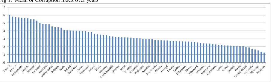
Figure 1 shows an overview of the corruption distribution for different countries. For each country
in the figure we calculated the mean over years (1984-2010). To the left with a high index value
(meaning low corruption risk) we find the Scandinavian countries and the three countries of
Oceania (Australia, New Zealand and Papua New Guinea). European countries in the dataset show
low/medium level of corruption while countries in Asia, Africa and South America have the highest
value.
3
The indices measuring corruption can be divided into two categories. One contains indices based on corruption perceptions; the other includes indices of experienced corruption.
4
ICRG table 3B, published by The PRS Group. 5
We display the autocorrelation matrix between the Corruption Index (CI), the Transparency International Index (TII) and Control of Corruption index (CCI), calculated over the 84 countries from 1996 to 2011 (we started from 1996 because of the availability of the TII and CCI).
CI TTI CCI
CI 1
TII 0.8693 1
CCI 0.8769 0.9781 1
6
http://www.prsgroup.com/ICRG_methodology.aspx 7
Even though the ICRG database includes a collection of records for about 150 countries, our analysis was performed on 75 countries. We avoided some countries because they were marginal with respect to our study.
8
8
Fig 1. Mean of Corruption index over years
This measure of corruption (like all corruption measures based on perception) has various
drawbacks (Lambsdorff, 2005); a significant gap between perception and facts being the major one .
The main regressor of the analysis is the Gallagher disproportionality (of the electoral outcome)
index; this is especially useful for comparing proportionality across electoral systems. The
Gallagher index (or least squares index) is a representation index of political parties within a
Parliament; it may be considered as a very good proxy for the measure of proportionality of an
electoral system because of the link between the kind of electoral system and the kind of political
parties representation.. Indeed, theoretical literature states (see Persson and Tabellini, 2000) that the
electoral system that guarantees a greater representation of political parties is a more proportional
one while the less representative one is less proportional. Blais (1988) confirmed that it is possible
to classify electoral systems according to their electoral outcomes. Moreover, empirical studies have
shown that a majoritarian system produces a higher level of dis-proportionality than a proportional
representation system (Lijphart, 1994; Anckar and Akademi, 2001), whereas a mixed-electoral
system produces an intermediate level (Powell and Vanberg, 2000; Anckar and Akademi, 2001).
Therefore, the Gallagher index is an excellent proxy for the degree of dis-proportionality of the
electoral system.9 The Gallagher index (thereafter GI) is constructed as
= 12 ( − )
where vi and si are respectively the share of votes and of seats of a single political party (i=1,....,n
political parties) at elections in each country in the time span under consideration. The index can
take values from 0 to 100 with 0 indicating perfect proportionality between seats and votes and 100
meaning that the only seat at stake goes to the winner. Clearly the bounds of the GI (0 and 100) are
only theoretical values. The GI between the investigated countries ranges from 0.26 to about 33.10
In this range fall the countries that have experienced plurality, PR and mixed systems as shown in
9
Dis-proportionality means the deviation of the parties’ seat shares from their vote shares. Perfect proportionality is the
situation in which each party receives exactly the same share of seats for the share of votes it receives. 10
See table 1 (Appendix) for the descriptive statistics of all variables.
9
table 2 (Appendix). In the time span 1980-2011, some countries maintained the same electoral
system, while other countries changed it. For example, Italy held a PR system from 1980 to 1993
and then a mixed one; Ukraine experienced all three systems: plurality 1994-1997, mixed
1998-2003 and PR since 2004. The concentration of mixed systems has been particularly pronounced in
post-communist Europe, where six states (in the database) currently employ systems of this type -
Romania, Lithuania, Hungary, Croatia, Poland and Albania. The majority of countries adopted PR
and then a mixed representation, with the minority using plurality rules. Not all the countries in the
dataset had democratic elections after 1980. Table 3 (Appendix) lists countries, in decades, from
their first democratic election; the majority of countries have had democratic elections since the
‘80s, and only two countries since 2000.11 Finally, in table 4 (Appendix), we provide the descriptive
statistics of GI according to the three electoral rules. It can be noticed that the mean of GI within PR
is lower than that within the mixed system and, in its turn, is lower than that within plurality; it
confirms that GI is a good proxy for electoral systems. But it can happen that, for the same value of
GI, electoral systems overlap. This happens because the GI is a proper representation index.
An important issue here is to deal with the possibility of endogeneity of the Gallagher index. All the
theoretical literature analysing the link between electoral rules and corruption considers the first as a
determinant of corruption and not the reverse. The endogeneity problem may arise when dealing
with political institutions, not the electoral system (this is the reason why the variable law_order -
that we will describe in the following paragraph - which controls for this kind of feature - is also
considered endogenous). In this respect, two other considerations must be made: 1) it seems
unlikely to think that the perception of corruption (as a menace to foreign investments) may affect
the way in which electoral systems are was
affected by corruption, the choice of one electoral rule rather than another would be a statement of
corruption for incumbent politicians, and they would risk dismissal from office. Therefore, we can
rule out the endogeneity issue of the dis-proportionality index.
The literature studying the causes of corruption names a long list of variables, claimed as
statistically significant determinants. They can be divided into four groups: 1) economic and
demographic, 2) political, 3) judicial and bureaucratic, 4) religious and geo-cultural (de Haan and
Seldadyo, 2005).12 A typical empirical study limits its attention to a small number of variables of
particular interest. Unfortunately, it is almost impossible to find the “true determinants” of
corruption: a variable found significant in a particular specification of the model, becomes
insignificant in an alternative model, or when other variables are incorporated. In order to overcome
11
it is clear that before the first year of a democratic election, GI shows missing values. 12
10
this drawback, Sala-i-Martin (1997) proposed to use a Sensitivity Analysis to establish which of the
potential determinants are robustly correlated with corruption.
In the choice of control variables we take a cue from the findings of the Sensitivity Analysis.
Therefore, in the empirical model, we firstly include the two typical controls in cross-country
analysis, the (log of) per capita GDP and the population size and secondly, in order to test the
robustness of results, we add a set of control variables believed as the most robust determinant of
corruption. The full list of control variables is the following:13
- Per capita GDP, in natural log (thereafter lngdp): it controls for structural differences in
economic development (de Haan and Seldadyo, 2005). By far the strongest and most consistent
finding of the new empirical work is that lower perceived corruption correlates closely with higher
economic development (La Porta et al. 1999, Ades & Di Tella 1999, Treisman 2000) and it can be
found in each region of the world (Treisman 2007),Kaufmann et al. (1999) and Hall and Jones
(1999) question the causal relationship between corruption and income: the per capita GDP is high
because of low corruption. For this reason we treat lngdp as endogenous.
- Population (thereafter pop): it controls for size. Empirical literature found contrasting evidence
(Knack and Azfar, 2003; Tavares, 2003).
- Government stability (thereafter gov_stab): it controls for quality of government. The higher the
quality of government, the lower the probability of corruption (de Haan and Seldadyo, 2005).
- Democratic accountability (thereafter dem): it controls for the level of democracy of a country.
There is a general consensus that democracy reduces corruption (de Haan and Seldadyo, 2005).
- Law and Order (thereafter law_order): it controls for the rule of law as a measure of the
confidence that agents have in the rules of society, the effectiveness of judiciary and the
enforceability of contracts (de Haan and Seldadyo, 2005). A stronger rule of law reduces the
likelihood of corruption taking place. Also in this regard, an issue of causality may emerge:
agents may trust the rule of law because corruption is low. In order to take this problem into
account, some estimations treat law_order as endogenous.
- Women (thereafter wom): it is the proportion of seats held by women in national parliaments
(%); it controls for the gender dimension of corruption. Conventional wisdom states that women
in public life can be an effective anticorruption strategy because women are less corruptible than
men. While the concept of women inherently possessing a higher level of integrity has been
challenged, studies have confirmed that there is a link between higher representation of women
in government and lower levels of corruption (Dollar et al., 1999; Goetz, 2004; Sung, 2003).
13
11
- General government consumption expenditure (thereafter G) – in % of GDP: it controls for
government size. There is no consensus among authors on the theoretical relationship between
government size and corruption (Fisman and Gatti, 2002; Bonaglia et al., 2001; Ali and Isse,
2003). Moreover, in order to consider a possible endogeneity of government sector size, in some
estimations we treat G as endogenous.
- Net enrollment primary rate, in natural log (thereafter lnschool): it controls for human capital
development. Empirical literature found contrasting evidence (Ali and Isse, 2003; Frechette,
2001).14
We follow the standard practice of counting a country as democratic according to its rate of Polity
IV political freedom score. Polity IV provides data on democracy level and regime duration. The
Polity IV index is a combined polity score ranging from -10 (strongly autocratic) to +10 (strongly
democratic), arrived at by subtracting the autocracy score from the democracy score. The democracy
and autocracy indexes were originally constructed additively based on the following indicators:
competitiveness of executive recruitment, openness of executive recruitment, constraints on the chief
executive, regulation of participation and competitiveness of participation. Scholars have reduced
the index to a dichotomous measure of democracy and autocracy. Two different thresholds are
frequently used for this purpose: the strictest measure defines countries which score 6 or higher on
the combined index (Raknerud and Hegre, 1997) as democratic, whereas more lenient studies have
taken score 3 as their threshold (Gleditsch and Hegre, 1997). In this work, we follow the latter
example and define as a democracy the countries whose score of Polity IV index is greater than +3
in the year of election.
4. Econometric specifications and results
The empirical analysis is twofold: parametric and semi-parametric
4.1 Parametric and semi-parametric analysis
We start with a description of the parametric specification of the model. In order to test the
hypothesis specified in section 2 we choose a cubic specification of the link between corruption and
the proportionality degree of the electoral system as the more general nonlinear function. Therefore,
the estimated equation is
, = , + + + + , + + + , (1)
of country I at time t; αi is a country-specific effect, µt is a time-specific effect. Two lags of the
dependent variable are introduced in the estimated equation because of the dynamic of corruption.15
14
12
Indeed, previous empirical analyses on corruption consider corruption as a dynamic phenomenon,
where past levels of corruption affect present levels (Aidt, 2003). The linear, quadratic and cubic
terms of GI catch the nonlinear specification of the model. The other regressors are those described
in the previous section.
Equation (1) is a dynamic panel data model which has been estimated using Arellano-Bover
(1995)/Blundell-Bond (1998) system GMM panel data techniques. The empirical analysis has been
conducted on a panel of 75 countries16 over 27 years (from 1984 to 2010).
The estimation results of the parametric analysis are in table 7 (Appendix). In order to control for
heteroskedasticity, every estimated equation has robust standard errors. The second-to-last row of
table 7 shows the Chi2 (and the p-value in parenthesis) of the Hansen test whose null hypothesis is
that over-identification restriction e do not reject the null and the model is correctly
specified.17 The last row of table 7 displays the p-value of the Arellano-Bond test for second-order
autocorrelation in the first differenced residuals: in all the specifications there is no autocorrelation
of residuals.
An attempt to overcome the limits of parametric analysis of non-linear models is strongly
recommended. A priori, we ignore any hint useful for the choice of a specific functional form. A
more general approach to the estimation of non-linear models is a non-parametric regression that
does not require the specification of the underlying functional form (Li and Racine, 2007).
The parametric analysis of corruption takes advantage of a rich econometric specification. A
dynamic model for panel data accounts for the persistence of corruption, its lagged response to
explanatory variables and residuals autocorrelation. Furthermore, some of the explanatory variables
can be endogenous. Non-parametric methods for panel data are not as well developed as the
parametric ones, and a dynamic model like (1) can hardly be estimated in a non-parametric setting.
It is well known how a full non-parametric analysis faces the “curse of dimensionality” given by the
rate of convergence of estimators being inversely related to the number of covariates. A widely
accepted answer to this problem is provided by semi-parametric models where some components
15
The estimation of equation (1) - without lags of corr - using fixed effect panel data techniques showed autocorrelation of residuals. In order to solve this problem, we introduced two lags of the dependent variable in the right-side of the equation (1).
16
Countries are: Albania; Argentina; Australia; Austria; Bahamas; Bangladesh; Belgium; Bolivia; Botswana; Brazil; Bulgaria; Canada; Chile; Costa Rica; Croatia; Czech Republic; Denmark; Dominican Republic; Ecuador; El Salvador; Finland; France; Germany; Greece; Guatemala; Guinea-Bissau; Guyana; Honduras; Hungary; Iceland; India; Indonesia; Ireland; Israel; Italy; Jamaica; Japan; South Korea; Lithuania; Luxembourg; Malta; Moldova; Mongolia; Mozambique; Myanmar; Namibia; Netherlands; New Zealand; Nicaragua; Norway; Papua New Guinea; Paraguay; Peru; Philippines; Poland; Portugal; Romania; Senegal; Slovakia; Slovenia; South Africa; Spain; Sri Lanka; Suriname; Sweden; Switzerland; Taiwan; Thailand; Trinidad & Tobago; Turkey; Ukraine; United Kingdom; United States; Uruguay; Zambia.
17
13
enter with a non-specified functional, while others are parametric. Here we apply the methods of
Baltagi and Li (2002) to the panel data model:
!, = "#, $ + %", & + + ', , ( = 1, … … , *; , = 1, … … , - (2)
where xi,t is a vector of explanatory variables, zi,t is a variable with a nonlinear relation to the
dependent variable, µi denotes fixed effects and νi,t are i.i.d random errors. The function g(zi,t) is not
specified.
Model (2) can be transformed by taking the first difference to eliminate individual fixed effects. The
new equation contains a non-linear component g(zi,t)-g(zi,t-1) that represents the main problem for
model estimation. The solution advanced by Baltagi and Li (2002) is to approximate g(z) with the
series pk(z), where pk(z) is the vector of the first k approximating functions. This implies that g(zi,t)
-g(zi,t-1) is approximated by pk(zi,t)-pk(zi,t-1). Spline functions are among the most used to approximate
an unknown function. Splines are piece-wise polynomial functions defined over intervals of the
support of z delimited by 1,...,k knots. The methodology advanced by Baltagi and Li (2002)
proceeds with the estimation of the parameter vector γ with the series method. This estimate is used to build an estimate of the error component νi,t that becomes the dependent variable in the non-parametric estimation of g(zi,t).
We use this panel regression method to estimate a model of cross-country corruption where we
distinguish a non-parametric component g(GIi,t) and a linear relationship between a set of control
variables and the corruption index. In order to concentrate our analysis on the non-parametric
relationship, we make some simplifying specification choices. The model is static, aiming at an
estimation of the long-run relationship. Questions with omitted dynamics are tackled with the use of
country time series made up of five-years averages and the introduction of time dummies among
regressors. The use of time averages also has the advantage of reducing the attenuation bias which
derives from possible measurement errors in the variables.
4.2 Results
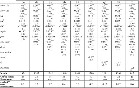
Column (a) in table 7 shows the estimation of equation (1) only with lngdp and pop. The
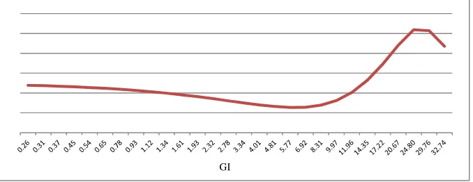
coefficients of GI, GI2 and GI3 are all highly significant, as well as the two lags of corr and lngdp. In order to graph the effect of the GI index on corruption, we use the following long-run equation:
= −0.190.23 +0.0170.23 −0.000380.23 +0.1390.23 45 67 (3)
In figure 1 below, on the horizontal axis we have constructed a scale of disproportionality index
14
value; then we calculate the Corruption index according to equation (3) using the estimated
[image:15.612.81.420.117.248.2]coefficients of GI, GI2, GI3and lngdp (the coefficient of pop is not significant).
Figure 1:Parametric fit of the relationship between corruption and the Gallagher Index
From the graph above, it emerges that the relationship between the proportionality degree of
electoral system and corruption has a minimum and maximum value. The value of GI which
maximises the Corruption index (that is, which minimises the level of corruption) is about 20, while
the value of GI which minimises the Corruption index (that is, which maximises the level of
corruption) is about 8. This shape of the proportionality degree-corruption relationship offers an
interesting interpretation. Initially, moving from the extreme left of the horizontal axis towards the
right, while the proportionality degree of the electoral system slightly reduces, the Corruption index
decreases (corruption increases) to its minimum value. It is reasonable to believe that this happens
because the electoral rule remains proportional, even though the proportionality degree of the
electoral system changes. Indeed, the PR degree of proportionality may vary according to factors
such as the precise formula used to allocate seats18, the number of seats in each constituency or in
the elected body as a whole19, and the level of any minimum threshold for election. Therefore,
reducing the proportionality degree of the electoral rule within PR systems (that is, without adding
some majoritarian elements) implies the reduction of the monitoring power of opponents without
introducing the voters’ monitoring on incumbent politicians - that means fertile ground for corrupt
actions: in figure 1 Corruption index decreases (corruption increases). Instead, when the GI starts
increasing (for example, it goes beyond 8, according to our estimations), it is also reasonable to
believe that the corresponding electoral system has become mixed. This means that the monitoring
power of opponents (ensured by PR elements) is reinforced by that of voters’ (ensured by plurality
elements): the effects of responsiveness of PR and accountability of majoritarian representation, put
18
Ranking PR formulas have been approached both theoretically (Gallagher 1992; Lijphart 1986; Loosemore and Hanby 1971) and empirically (Gallagher 1991; Blondel 1969). The most widely accepted ranking is Lijphart’s (1986), which considers the Hare and Droop largest remainder (LR) methods to be the most proportional, followed by the Sainte-Lagu¨e highest-average (HA) method, followed by Imperiali LR, d’Hondt HA, and Imperiali HA. A critical re-examination of the ranking of electoral formulas was proposed by Benoit (2000).
19
Generally, the wider the district magnitude, the more proportional the PR is.
15
together, are stronger at fighting corruption. This can be clearly seen in figure 1 starting from the
GI s to grow as the GI rises up to the value of about 20 which
maximises the Corruption index. After reaching its maximum, the Corruption index decreases
again. It is interesting to underline that in the increasing section of the Corruption index in figure 1
(which corresponds to the interval of GI [8-20]), the small reduction in the proportionality degree of
mixed rule implies that the marginal substitution between the monitoring power of opponents in
favour of the monitoring power of voters is beneficial in fighting corruption. While considering
mixed electoral rules with a proportionality degree always lower (GI>20), the same marginal
substitution leads to a corruption increase: this happens because the monitoring power of opponents
almost disappears. As figure 1 shows, we can find a value of the GI which maximises the
Corruption index (meaning minimising the level of corruption). This suggests that the “best”
proportionality degree that a mixed system should have must almost equally balance the voters’ and
the opponents’ monitoring power in order to maintain their independence and re-enforce each other.
This result remains robust with the introduction of all the control variables that we listed above, as
shown in table 7.
Where significant, Lngdp is positive as expected, meaning that a greater level of economic
development is correlated to less perceived corruption. Pop, instead, is never significant. Starting
from column (b) we introduce gov_stab: it is always significant (except in specification (i)) and
positive, as expected - the higher the quality of government, the lower the corruption. The same
happens for dem, from specification (c): it is always positive and significant (except in (i)) - the
greater the level of democracy of a country, the lower the level of corruption. Law_order controls
for the rule of law: in specification (d) it is treated as exogenous and its sign is positive and
significant - a stronger rule of law reduces the likelihood of corruption. In order to take into account
the issue of causality of this variable, in specification (e) we treat it as endogenous - the result does
not change. Columns (f) and (i) show that women and lnschool are not significant. Public
consumption spending shows a positive and significant coefficient in (g) - the larger the relative
size of public sector, the lower the likelihood of corruption; this coefficient becomes insignificant if
G is treated as endogenous as in (h).
The estimation of the parametric model (1) provided us with a peculiar non-linear relationship
between the Gallagher disproportionality index and the Corruption index. We conducted a
parametric in order to confirm this particular functional form. As in the parametric model, the
semi-parametric one considers the variable of interest GI entering the regression equation as exogenous.
However, we depart from that econometric specification by including in the linear component of the
16
theoretical and applied literature. In particular, this is the case of democratic accountability (dem),
government stability (gov_stab), proportion of seats held by women in national parliaments (wom),
and the population (pop). Table 8 (Appendix) presents the results of the estimation of five
specifications of the model. All the specifications include time dummies to account for shifts in the
relationships over the period 1984-2010. As Desbordes and Verardi (2012) have done, we use
B-splines both as base functions pk(GI) and to estimate g(GIi,t).
20
In the baseline estimates (a’), the linear regressors are time dummies. Other regressions see the
addition of one variable at a time. Estimates confirm that democratic accountability and government
stability are significant explanatory variables of corruption.
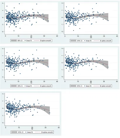
Figure (2) shows the plot of the non-parametric estimate of g(GIi,t) for each of the five
specifications of the parametric component of the model. In particular, each panel displays the plot
of the relation between Corr and GI net of the fixed effects and the linear part of the regression
equation.21 In each graph the shaded area displays confidence intervals at 95% level of confidence.
The five plots of the estimate of the function g(GIi,t) show almost the same shape: a U followed by
an inverted U. Hence, we find a substantial confirmation of the main result of the parametric
analysis. As the graphs display, the results are confirmed not only by their shape, but also by their
values. That is, the min and max of the Corruption index in the semi-parametric analysis fall
approximately at a GI=8 and a GI=20 respectively, similar to the findings of the parametric
analysis. This emphasises even more the robustness of the relationship that we found between the
proportionality degree of electoral rules and corruption.
20
Computations were made using the STATA command xtsemipar by François Libois and Vincenzo Verardi (2013). 21
17
Figure 2: Non-parametric fit of the relationship between corruption and the Gallagher Index. Partial residuals centred around the mean.
5. Concluding remarks
This work offers a parametric and semi-parametric analysis of the relationship between the
proportionality degree of an electoral system and corruption. The use of the Gallagher
dis-proportionality index as a measure of the dis-proportionality degree of an electoral rule has allowed us
to properly consider mixed electoral systems alongside the two traditional ones, PR and plurality.
Given that mixed rules are becoming the preferred choice of more and more governors, it seems
18
the gap empirical literature has in this field. Results confirm our theoretical framework and show
that the relationship between the proportionality degree and corruption is not linear. Graphically,
this relationship appears as a sine curve, with the Corruption index reaching its minimum at low
values of GI, and its maximum at high values of GI. The policy implications of this result are
newsworthy. Even though PR allow their proportionality degree to be modified through the
variation of the electoral formula or the introduction of some thresholds, the reduction of the
proportionality degree within the same PR is not beneficial in fighting corruption. Indeed, this kind
of system weakens the monitoring power of opponents (because the representativeness reduces)
without the introduction of the voters’ monitoring. On the contrary, the contamination of the PR
with plurality elements (therefore, the switch to mixed rules), allows both monitors to exercise their
power to induce politicians to avoid corrupt behaviour. Increasing plurality elements into mixed
systems is beneficial only up to certain proportionality degrees after this the corresponding level of
corruption begins to grow. For governors who want to adopt mixed electoral systems, their choice
of proportionality degree becomes, therefore, fundamental. Further studies are needed in helping
19
[image:20.612.79.368.96.429.2]Appendix
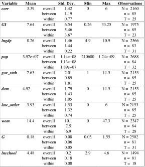
Table 1: Statistics
Variable Mean Std. Dev. Min Max Observations
corr 3.39 overall 1.42 0 6 N = 2160
between 1.19 n = 85
within 0.77 T = 25
GI 7.64 overall 6.54 0.26 33.25 N = 1975
between 5.46 n = 85
within 3.67 T = 23
lngdp 8.26 overall 1.46 4.9 10.9 N = 2566
between 1.44 n = 83
within 0.22 T = 31
pop 3.97e+07 overall 1.14e+08 210600 1.24e+09 N = 2688
between 1.13e+08 n = 84
within 1.89e+07 T = 32
gov_stab 7.63 overall 2.01 1 11.5 N = 2153
between 0.89 n = 85
within 1.81 T = 25
dem 4.92 overall 1.79 0 11.5 N = 2153
between 1.43 n = 85
within 1.05 T = 25
law_order 3.93 overall 1.53 0 6 N = 2153
between 1.32 n = 85
within 0.74 T = 25
wom 14.4 overall 10.1 0 47.3 N = 2347
between 7.5 n = 84
within 6.9 T = 28
G 0.18 overall 0.08 0.03 1.55 N = 2502
between 0.06 n = 81
within 0.05 T = 31
lnschool 4.48 overall 0.2 2.9 4.6 N = 1494
between 0.18 n = 81
within 0.08 T = 18
Table 2: Distribution of countries according to their electoral system, 1980-2011
PR Mixed Plurality
Argentina, Austria, Belgium, Costa Rica, Denmark, Ecuador El Salvator (since 1998 ), Finland, Guinea-Bissau (Since 2007), Guyana, Iceland, Indonesia, Ireland, Israel, Italy (since 1980 to 1993), Luxembourg, Malta, Moldova (since 1994), Mongolia 2009, Mozambique
(since 1995), Namibia (since 1989),
Netherlands, Nicaragua (since 1987), Norway, Paraguay, Peru (since 1981), Poland (since 1990 to 2006), Portugal, Luxembourg, Malta, Moldova (since 1994), Mongolia 2009, Mozambique (since 1995), Namibia (since 1989 ), Netherlands, Nicaragua (since 1987), Norway, Paraguay, Peru (since 1981), Poland (since 1990 to 2006), Portugal, Romania (since 1991 to 2006), Slovakia (since 1993), Slovenia (since 1992), South Africa, Sri Lanka, Suriname (since 1988), Sweden, Turkey (since 1984), Ukraine (since 2007), Uruguay (since 1985).
Albania (since 1992), Australia, Bolivia (since 1983), Brazil, Croatia (since 1993), Czech Rep. (since 1991), Dom. Rep., El Salvador (since 1983 to 1997), Germany, Greece, Guatemala (since 1986), Honduras (since 1982), Hungary (since 1991), India, Italy (since 1994),
Japan, Lithuania (since 1993),
Mozambique (in 1994), New Zealand (since 1993), Philippines (since 1999), Poland (since 2007), Romania (since 2007), Senegal, South Korea, Spain, Suriname (1980), Switzerland, Taiwan (since 1992), Ukraine (since 1998 to 2003)
Bahamas, Bangladesh, Botswana,
Canada, Chile (since 1990), France, Jamaica, Mongolia (since 1993 to 2008), New Zealand (since 1980 to 1992), P. N. Guinea, Philippines (since 1988 to 1997), Thailand, Trinidad-Tobago, Ukraine (since 1994 to 1997), UK, USA, Zambia (since 1992)
20
Table 3: list of countries, in decades, from their first democratic election
1980-2001 1990-2011 2000-2011
Argentina, Australia, Austria, Bahamas, Belgium, Bolivia, Botswana, Brazil, Bulgaria, Canada, Chile, Costa Rica, Denmark, Dominican Republic, Ecuador, El Salvador, Finland, France, Germany, Greece, Guyana, Honduras, Iceland, India, Ireland, Israel, Italy, Jamaica, Japan, South Korea, Luxembourg, Malaysia, Malta, Namibia, Netherlands, New Zealand, Norway, Papua New Guinea, Paraguay, Peru, Philippines, Portugal, Senegal, Spain, Sri Lanka, Suriname, Sweden, Switzerland, Taiwan, Thailand, Trinidad & Tobago, Turkey, United Kingdom, United States, Uruguay
Bangladesh, Czech Republic, Guatemala, Guinea-Bissau, Indonesia, Hungary, Indonesia, Lituania, Moldova, Mongolia, Myanmar, Mozambique, Nicaragua, Poland, Romania, Russia, Slovakia, Slovenia, South-Africa, Ukraine, Zambia
Albania, Croatia
Table 4: GI statistics according to electoral systems, 1980-2011
PR MIXED PLURALITY
Mean Std. Dev. Min Max Mean Std. Dev. Min Max Mean Std. Dev. Min Max
[image:21.612.75.523.313.667.2]4.6 4.4 0.26 29.4 7.8 4.9 0.91 30.2 14.4 7.5 1.3 33.25
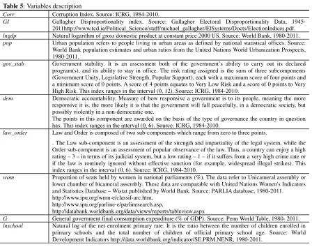
Table 5: Variables description
Corr Corruption Index. Source: ICRG, 1984-2010.
GI Gallagher Disproportionality index. Source: Gallagher Electoral Disproportionality Data,
1945-2011http://www.tcd.ie/Political_Science/staff/michael_gallagher/ElSystems/Docts/ElectionIndices.pdf.
lngdp Natural logarithm of gross domestic product at constant price 2000 US. Source: World Bank, 1980-2011.
pop Urban population refers to people living in urban areas as defined by national statistical offices. Source:
World Bank population estimates and urban ratios from the United Nations World Urbanization Prospects, 1980-2011.
gov_stab Government stability. It is an assessment both of the government’s ability to carry out its declared
program(s), and its ability to stay in office. The risk rating assigned is the sum of three subcomponents (Government Unity, Legislative Strength, Popular Support), each with a maximum score of four points and a minimum score of 0 points. A score of 4 points equates to Very Low Risk and a score of 0 points to Very High Risk. This index ranges in the interval (0, 12). Source: ICRG, 1984-2010.
dem Democratic accountability. Measure of how responsive a government is to its people, meaning the more
responsive it is, the more likely it is that the government will fall peacefully, in a democratic society, but possibly violently in a non-democratic one.
The points in this component are awarded on the basis of the type of governance the country in question has. This index ranges in the interval (0, 6). Source: ICRG, 1984-2010.
law_order Law and Order is composed of two sub-components which range from zero to three points.
. The Law sub-component is an assessment of the strength and impartiality of the legal system, while the Order sub-component is an assessment of popular observance of the law. Thus, a country can enjoy a high rating – 3 – in terms of its judicial system, but a low rating – 1 – if it suffers from a very high crime rate or if the law is routinely ignored without effective sanction (for example, widespread illegal strikes). This index ranges in the interval (0, 6). Source: ICRG, 1984-2010.
wom Proportion of seats held by women in national parliaments (%). The data refer to Unicameral assembly or
lower chamber of bicameral assembly. These data are comparable with United Nations Women's Indicators and Statistics Database – Wistat published by World Bank. Source: PARLIA database, 1980-2011. http://www.ipu.org/wmn-e/classif-arc.htm,
http://www.ipu.org/parline-e/parlinesearch.asp,
http://databank.worldbank.org/data/views/reports/tableview.aspx
G General government final consumption expenditure (% of GDP). Source: Penn World Table, 1980- 2011.
lnschool Natural log of the net enrolment primary rate. It is the ratio between the number of children enrolled in
21
Table 6: Correlations
GI lngdp pop gov_stab dem law_order wom G lnschool
GI 1
lngdp -0.22
pop -0.009 -0.12 1
gov_stab 0.02 0.11 -0.009 1
dem -0.24 0.39 0.04 0.20 1
law_order -0.15 0.66 -0.06 0.17 0.46 1
wom -0.35 0.31 -0.14 0.16 0.26 0.30 1
G 0.08 -0.11 -0.07 -0.03 0.06 0.04 -0.03 1
lnschool -0.13 0.53 -0.02 -0.06 0.34 0.27 0.12 0.09 1
Table 7: Estimations
(a) (b) (c) (d) (e) (f) (g) (h) (i)
corr(-1) 1.02***
(17) 1.00*** (15) 0.9*** (13) 0.9*** (13) 0.9*** (18) 1.0*** (15) 0.9*** (12) 0.9*** (13) 0.9*** (12)
corr(-2) -0.25***
(-6) -0.23*** (-5) -0.23*** (-5) -0.24*** (-6) -0.22*** (-6) -0.24*** (-6) -0.22*** (-5) -0.22*** (-5) -0.22*** (-5)
GI -0.19***
(-2.3) -0.21*** (-2.4) -0.22*** (-2.5) -0.21*** (-2.5) -0.09** (-2.06) -0.13** (-2.2) -0.30*** (-2.45) -0.30*** (-2.6) -0.2** (-2.05)
GI2 0.017**
(2.2) 0.018** (2.3) 0.02** (2.4) 0.018** (2.3) 0.007* (1.8) 0.01** (2) 0.02** (2.3) 0.02** (2.5) 0.01** (1.97)
GI3 -0.0003**
(-2.1) -0.0004** (-2.2) -0.0004** (-2.2) -0.0004** (-2.2) -0.0001* (-1.7) -0.0002* (-1.8) -0.0006** (-2.13) -0.0006** (-2.3) -0.0004* (-1.8)
lngdp 0.13***
(3.2) 0.13*** (3.1) 0.125*** (2.9) 0.05 (1.07) 0.02 (0.7) 0.09** (2.3) 0.14*** (3) 0.15*** (2.6) 0.02 (0.35)
pop 1.79e-10
(1.2) 1.90e-10 (1.4) 1.72e-10 (1.3) 7.39e-11 (0.6) 4.76e-11 (0.5) 6.47e-11 (0.5) 2.32e-10 (1.6) 2.55e-10 (1.3) 4.09e-11 (0.3)
gov_stab 0.04**
(2.3) 0.03*** (1.9) 0.02** (1.9) 0.03** (2.37) 0.04*** (3.3) 0.05*** (2.9) 0.05** (2.44) -0.002 (-0.08)
dem 0.05**
(2.1) 0.03* (1.85) 0.03* (1.8) 0.04** (1.98) 0.05** (2.3) 0.05** (2.2) 0.03 (1.35)
law_order 0.1**
(2.3)
0.1**
(2.08)
0.14**
(2.1)
wom -0.002
(-0.7)
G 0.92**
(2.17)
1.48 (0.5)
lnschool -0.1
(-0.2)
N. obs. 1374 1342 1342 1340 1404 1299 1294 1294 945
Chi2 (p-value) Hansen test 35 (0.9) 33 (0.9) 34 (0.9) 34 (0.9) 45 (0.9) 33 (0.9) 32 (0.9) 32 (0.9) 41 (0.98
p-value 2nd
order autocorrelation
0.2 0.2 0.2 0.4 0.6 0.2 0.13 0.12 0.6
Notes. All regressions contain calendar year dummies (results not reported); the time span is 1984-2010. The dependent variable is
corr. Standardised normal z-test values are in parentheses; robust standard errors. In column (e) and (h) law_order and G respectively
[image:22.612.78.538.243.537.2]22
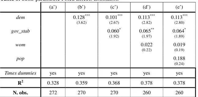
Table 8: Semi-parametric Fixed Effects Estimation
(a’) (b’) (c’) (d’) (e’)
dem 0.128***
(3.62)
0.101***
(2.67)
0.113***
(2.82)
0.113***
(2.80)
gov_stab 0.060*
(1.92)
0.065**
(1.97)
0.064*
(1.89)
wom 0.022
(0.22)
0.019 (0.19)
pop 0.188
(0.24)
Times dummies yes yes yes yes yes
R2 0.328 0.359 0.368 0.378 0.378
N. obs. 272 270 270 260 260
Notes. The dependent variable is corr. All regressions contain a non-parametric function of the Gallagher Disproportionality Index
23
References
Abdiweli M. Ali, Hodan S. Isse, (2003), Determinants of Economic Corruption:A Cross-Country Comparison, Cato Journal, vol. 22, n.3, pp. 449-466.
Ades, A., Di Tella, R. (1999), Rents, Competition, and Corruption, American Economic Review, vol. 89, n.4, pp. 982-92.
Aidt, T.S., (2003), Economic Analysis of Corruption: A Survey, in The Economic Journal, vol. 113, pp. 632-652.
Anckar, C., Akademi, A. (2001), Effects of electoral systems. A study of 80 countries. Working Paper presented at the SNS Seminar in Stockholm.
Baltagi, B. H., Li D.,(2002), Series Estimation of Partially Linear Panel Data Models with Fixed Effects, Annals of Economics and Finance, 3, pp. 103-116.
Bardhan, P., Yang, T. (2004), Political Competition in Economic Perspective, Bureau for Research and Economic Analysis of Development, Working Paper 78.
Benoit, K., (2000), Which Electoral Formula Is the Most Proportional? A New Look with New Evidence, Political Analysis, vol. 8,n. 4, pp. 381-388.
Blais, A. (1988), The classification of electoral systems. European Journal of Political Research, vol. 16, pp. 99-110.
Blondel, J.,(1969), An Introduction to Comparative Government. London: Weidenfeld and Nicholson.
Blundell, R. e Bond, S. (1998), GMM Estimation with Persistent Panel Data: An Application To Production Functions, Institute for Fiscal Studies, Working Paper Series, n. 99/4.
Boix, C. (2003), Democracy and Redistribution. Cambridge: Cambridge University Press.
Bonaglia, F. de Macedo, J.B., Bussolo, M., (2001), How Globalization Improves Governance,
Discussion Paper n. 2992, Centre for Economic Policy Research, Organization for Economic Co-operation and Development, Paris, France.
Chang, E. C. C., Golden, M. (2007), Electoral systems, district magnitude and corruption, British Journal of Political Science, vol. 37, pp.115–137.
Chang, E. C.C. (2005), Electoral Incentives for Political Corruption under Open-List Proportional Representation, Journal of Politics, vol. 67, n. 3, pp.716-30.
de Haan, J. and H. Seldadyo (2005), The Determinants of Corruption: A Reinvestigation, unpublished paper prepared for the EPCS-2005 Conference Durham, England, 31 March–3 April 2005.
de Haan, J. Sturm, J.E.(2005), Determinants of Long-term Growth: New Results Applying Roboust Estimation and Extreme Bounds, TWI Research Paper Series n. 12, Thurgauer Wirtschaftsinstitut, Universität Konstanz.
Desbordes R.,Verardi V., (2012), Refitting the Kuznets Curve. Economics Letters, 116, pp. 258-261.
Dollar D., Fisman R., Garri R.(1999), Are Women Really the Fairer Sex? Corruption and Women in Government, World Bank Working Paper Series, n. 4.
24
Forejohn, J. (1986), Incumbent performance and electoral control, Public Choice, vol. 50 pp. 5-25.
Frechette, G. R. (2001), A Panel Data Analysis of the Time-Varying Determinants of Corruption,
Paper presented at the EPCS.
Gagliarducci, S., Nannicini, T., Naticchioni, P. (2011), Electoral Rules and Politicians’ Behavior: A Micro Test, American Economic Journal: Economic Policy, vol. 3, n. 3, pp. 144-174.
Gallagher, M. (1992), Comparing Proportional Representation Electoral Systems: Quotas, Threshol ds, Paradoxes and Majorities, British Journal of Political Science, vol. 22, pp. 469-496.
Gallagher, M. (1991), Proportionality, Disproportionality and Electoral Systems, Electoral Studies
vol. 10, n. 1, pp. 33-51.
Gleditsch, N.P., Hegre, H. (1997), Peace and Democracy: Three levels of Analysis, Journal of Conflict Resolution, vol. 41, n. 2, pp. 283-310.
Goetz, A. (2004), Political Cleaners: How Women are the New Anti-Corruption Force. Does the Evidence Wash?, available online at http://www.u4.no/document/showdoc.
Golden, M. A., Chang E. C. (2001), Competitive Corruption: Factional Conflict and Political Malfeasance in Postwar Italian Christian Democracy, World Politics, vol. 53, n. 4, pp.588-622.
Hall, R. E. Jones, C. I. (1999), Why do Some Countries Produce so much more Output per Worker than Others, Quarterly Journal of Economics, vol. 114, pp. 83-116.
Huntington, S.P. (1968), Political Order in Changing Societies, New Haven: Yale University Press.
Jain, A. K. (2001), Corruption: A Review, Journal of Economic Surveys vol. 15, n. 1, pp. 71–121.
Kaufmann, D. Kraay, A., Mastruzzi, M. (1999), Governance Matters, World Bank Policy Research Working Paper, n. 2196.
Knack, S., Azfar, O. (2003), Trade Intensity, Country Size and Corruption, Economics of Governance, vol. 4, pp. 1-18.
Kostadinova, T. (2002), Do Mixed Electoral Systems Matter?: A Cross-National Analysis of their Effects in Eastern Europe. Electoral Studies vol.21, n.1, pp. 23-34.
Kunicova, J. Rose-Ackerman, S. (2005), Electoral Rules and Constitutional Structures as Constraints on Corruption, British Journal of Political Science, vol. 35, n.4, pp.573–606.
La Porta, R., Lopez-de-Silanes, F., Shleifer, A., Vishny, R.W. (1999), The Quality of Government,
Journal of Law, Economics, and Organization, vol. 15, pp. 222-79.
Lambsdorff, J. G. (2005), Consequences and Causes of Corruption: What do We Know from a Cross-Section of Countries?, University of Passau, Passau.
Leff, N. H. (1964), Economic Development through Bureaucratic Corruption, The American Behavioral Scientist, vol. 8, n.3, pp. 8-14.
Li Q., Racine J. S., (2007), Nonparametric Econometrics. Theory and Practice, Princeton University Press, Princeton.
Libois F.,VerardiV., (2013) Semiparametric fixed-effects estimator, Stata Journal, 13, pp. 329-336.
Lijphart, A. (1986), Degrees of Proportionality of Proportional Representation Formulas, In Elector al Laws and Their Political Consequences, ed. Bernard Grofman and Arend Lijphart. New York: A gathon Press.