A SENSITIVITY ANALYSIS OF A DYNAMIC RESTRICTED EQUILIBRIUM MODEL 1
TO EVALUATE THE TRAFFIC NETWORK RESILIENCE 2
3 4 5
Beatriz Martinez-Pastor, Corresponding Author
6
Dept. of Civil, Structural and Environmental Engineering 7
Trinity College Dublin, Ireland 8
Tel: 00 353 (0) 899528639; Email: [email protected] 9
10
Maria Nogal 11
Dept. of Civil, Structural and Environmental Engineering 12
Trinity College Dublin, Ireland 13
Tel: 00 353 (0) 899861302; Email: [email protected] 14
15
Alan O’Connor 16
Dept. of Civil, Structural and Environmental Engineering 17
Trinity College Dublin, Ireland 18
Tel: 00 353 1896 1822; Email: [email protected] 19
20
Brian Caulfield 21
Dept. of Civil, Structural and Environmental Engineering 22
Trinity College Dublin, Ireland 23
Tel: 00 353 1896 2534; Email: [email protected] 24
25 26 27
Word count: 2,528 words text + 7 tables/figures x 250 words (each) = 4,278 words 28
29 30 31 32 33 34
ABSTRACT 1
Extreme weather events have a devastating impact on traffic networks. Therefore, mathematical 2
tools that are able to measure systematically the impacts of extreme weather events, i.e. to 3
evaluate its resilience, should be developed. With the aim of improving the resilience of a traffic 4
network when affected by a hazard, a profound knowledge of the model to evaluate resilience is 5
necessary. Consequently, the model parameters should be analized, since these parameters 6
represent the characteristics of the network and this analysis will permit to identify those 7
characteristics that should be improved to reach a more resilient system. This paper develops a 8
sensitivity analysis that reduces the number of studied point needed due to its statistical approach 9
using a global technique (Latin Hypercube), without losing efficiency, as a local technique 10
(One-At-a-Time) is applied too. This analysis confirms that the model to evaluate the resilience 11
represents the real behavior of the traffic network. The results show that the intensity of the 12
hazards is the most sensitive parameter. When hazard intensity is low, the impedance of the 13
system becomes the most sensitive parameter. 14
15 16 17
Keywords: Hazards, Extreme Weather, Vulnerability, Stress Level, Latin Hypercube, 18
On-At-a-Time, Local Sensitivity, Global Sensitivity. 19
INTRODUCTION 1
A variety of extreme weather events, including river floods, rain induced landslides, droughts, 2
winter storms, wildfire, and hurricanes, have threatened and damaged many different regions 3
worldwide. These events have a devastating impact on critical infrastructure systems resulting in 4
high social, economical and environmental costs. For this reason, it is imperative to develop a 5
mathematical tool that is able to measure systematically the impacts of extreme weather events 6
on transport networks. 7
The concept that evaluates the behavior of a traffic network when a perturbation takes place is 8
known as resilience. The most common definition of this holistic feature was given by Foster 9
(1993) as “the capacity to absorb shocks gracefully”.
10
With the goal of improving the resilience of a network when affected by a hazard, the 11
weaknesses of the system should be identified. Therefore, the knowledge of the most influential 12
variables involved in the model to evaluate the resilience, allows the enhancement of this 13
characteristic. With this aim, a sensitivity analysis is carried out. 14
A sensitivity analysis identifies the influence of each parameter on the outputs of the model, 15
permitting a profound knowledge of its behavior. In addition, the definition of the inputs will be 16
more efficient after studying how these parameters modify and influence the model. 17
Different methodologies to analyze the sensitivity have been developed previously. These 18
methods can be differentiated between local methods and global methods, the former focuses on 19
estimating the local impact of a parameter on the model outputs. 20
Whereas global techniques are based on sampling methods which scan, in a random or 21
systematic way, the complete range of the parameters involved in the model. Selection of the 22
sampling strategy is crucial to the sensitivity analysis. 23
The paper is organized as follows; Section 2 describes the model and the parameters involved. 24
Section 3 presents the analysis of sensitivity and its application. Finally, in Section 4 some 25
conclusions and future research lines are drawn. 26
27 28
THE MODEL AND THE PARAMETERS INVOLVED 29
When a disaster occurs, the traffic network is affected mainly through two different ways, 30
namely, (a) user travel costs (generally time) increase and (b) users become aware of these 31
greater costs and try to reduce them by changing their route choices, generating a certain stress 32
level in the network. When the alteration stops and the initial state is recovered, the travel costs 33
are recuperated and users eventually return to their initial route choices. On the other hand, if the 34
alteration stops but the initial state is not recovered, users will find other route choices that
35
minimize their costs, though these costs will be greater than before. The explained performance 36
is measured by the concept of resilience. Resilience can be defined as the capacity of a
37
transportation network (a) to absorb disruptive events, maintaining its level of service, and (b) to
38
return to a level of service equal to or greater than the pre-disruption level of service within a
39
reasonable time frame, Freckleton et al.(2012). In this paper only the resilience in the 40
perturbation stage is analyzed. 41
The assessment of the traffic network resilience requires a dynamic approach. With this aim, 42
Nogal et al. (2015) propose a “Dynamic Equilibrium-Restricted Assignment Model” (DERAM), 43
which allows the simulation of the network behavior when a disruptive event occurs. This 44
approach permits the inclusion of the stress level of the system together with the extra cost 45
generated by the hazard. This model proposes that the network behavior is restricted by a system 46
The perturbation resilience is defined between (0, 100), 100% being the optimum value. 1
Moreover, a cost threshold is included to assume the system break-down. This value restricts the 2
perturbation resilience and is the limit-state associated with the failure of the travel cost network 3
due to the extreme overcost generated by a strong perturbation. Although the system could 4
theoretically recover, it would imply an unacceptable effort by the system. 5
Furthermore, a travel cost function including climatological events has to be considered. More 6
precisely, Nogal et al. (2014) propose the following expression. 7
8
a
τ (t) = τ0a 1+maexp
Sa(t) βa
+pah(t) !
"
# $
%
&exp(−γa)
1−h(t) ( ) * * * * + , -. / 0 0 1 0 0 2 3 0 0 4 0 0 , 9 (1) 10 11
where τaand τ0aare denoted as the actual travel time and the free travel time, respectively; ma, 12
βaand γaare parameters related to the traffic characteristics; Sa(t) is the saturation degree 13
computed as the ratio between the actual flow and the capacity; h(t) is the hazard intensity 14
whose range is (0,1), and pa is the specific sensitivity of each link to a given hazard. For 15
instance, in the case of pluvial flooding, padepends on the catchment area, slope of the road, 16
type of pavement, existence of element of protection, etc. Subscript a implies association with 17 link a. 18 19 20 SENSITIVITY ANALYSIS 21 22 Methodology 23
The applied methodology is an integration of a local into a global sensitivity methodology. Based 24
on the complexity of the resilience model defined previously, this paper presents a combination 25
of One-At-a-Time (OAT) for the local sensitivity and Latin Hypercube (LH) sampling for a 26
global approach (Griensven et al (2006)). According to the OAT technique, the analysis is 27
performed by varying each parameter while the rest remainds constant. This local method is as 28
simple as efficient, however this process can become quite intensive with larger models. Then, 29
instead of applying it in a large number of points to cover the entire range of the parameters, a 30
global methodology has been chosen to obtain a sample of points that represents the different 31
variables. The selected global sampling procedure (LH) allows the reduction of the sample size. 32
Due to the importance of the pairing procedure, the method Translational Propagation algorithm 33
proposed by Viana et al (2010) has been implemented. The main advantage of this methodology 34
is that it requires virtually no computational time. When the sample is obtained, the local 35
sensitivity analysis can be accomplished as follows. Considering that the total space is covered 36
and the sample is a reliable and robust representation of the global, the resilience is evaluated for 37
each point of the sample. Then, every variable in each sample point is modified in a percentage 38
to calculate the corresponding resilience in that close point. It is important to modify only one 39
variable each time, in this way, the behavior of the modified variable is identified. Measuring the 40
The percentage applied for modifying the variable is also a critical point. Since, on the one hand,
1
small values can show the instabilities of the model, being this behavior not according with the 2
real tendency of the model. On the other hand, if this value is too large, the derivative loses its 3
meaning.
4
The formulation to assess the sensitivity is based on the concept of derivative, that is 5
6
ξ=Rd
+
(x,Y)−R(Z)
d , x,Y ∈Z, (2)
7
8
where Z is the set of variables involved in the model, x, is the modified variable and Y, the subset 9
of variables which remain constant. R is the resilience calculated for the initial parameter set Z 10
and Rd
+is the resilience calculated when one parameter has been increased by a percentage, d. 11
Sensitivity, denoted by ξ, is a dimensionless parameter. 12
13
Application of the Methodology 14
This methodology is applied in a simple traffic network to analyze the sensitivity of the set of 15
variables defined in section 2, that is Z= {α, !!, h(t), !!, !! }. 16
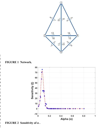
This traffic network consists of 5 nodes, 16 links and 9 routes, (see Figure1). The sensitivity 17
analysis is carried out by modifying the model parameters as shown in Table 1. It is noted that 18
only characteristics of links 13 and 16 change in each evaluation with the aim of distinguish the 19
effect. In this case, the sample size is 50 and the percentages of variation, dare 1, 5, 10%. 20
Figures 1-6 show the results associated with the percentage of 10%, as the results for the other 21
percentages follow a similar tendency. 22
[image:5.612.70.563.425.693.2]23
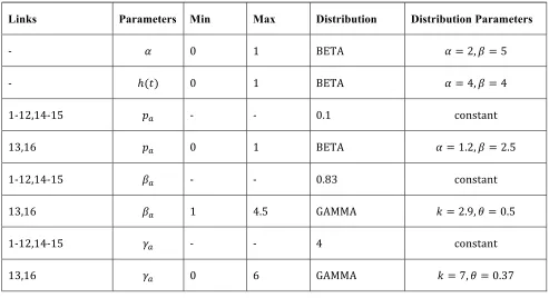
TABLE 1 Values and statistical distributions of the parameters. 24
25
26 27
Links Parameters Min Max Distribution Distribution Parameters
!" !" 0" 1" BETA" !=2,!=5"
!" ℎ(!)" 0"" 1" BETA" !=4,!=4"
1!12,14!15" !!" !"" !" 0.1" constant"
13,16" !!" 0" 1" BETA" !=1.2,!=2.5"
1!12,14!15" !!" !" !" 0.83" constant"
13,16" !!" 1" 4.5" GAMMA" !=2.9,!=0.5"
1!12,14!15" !!" !" !" 4" constant"
1 2
FIGURE 1 Network.
[image:6.612.227.374.60.275.2]3 4 5 6 7 8 9 10 11 12 13 14 15 16 17 18 19 20
FIGURE 2 Sensitivity of α . 21
22
The sensitivity of the parameters is analysedthrough the development of two cases, since the
23
influence of h(t) in the model is crucial. The first case shows the sensitivity of the variables when 24
the possible values of h(t)are smaller than 0.3, and in the second case, the values of h(t) are 25
higher. When h(t)takes higher values the model tends to reach the break point and the resilience 26
index becomes 0, therefore, the sensitivity of the rest of the parameters is negligible. These cases
27
are shown in the figures with red-circle points. 28
In lower values of h(t),the most sensitivite parameter is α, (see the sensitivity range in Figure 2).
29
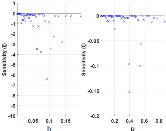
The influence of h(t)is larger than the influence of !! (see the sensitivity range in Figure 3-4). In 30
addition, the sign of the sensitivity in these two cases implies, as expected, that an increase in the 31
1
[image:7.612.77.353.75.294.2] [image:7.612.50.355.80.588.2]2 3
FIGURE 3 Sensitivity of h and p for small values of h. 4
5
6 7
FIGURE 4 Sensitivity of h and p for large values of h.
1 2
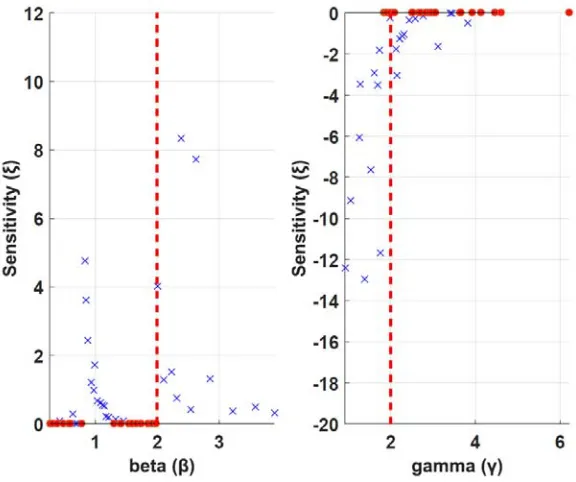
FIGURE 5 Sensitivity of βand γ for small values of h.
3 4 5
[image:8.612.76.364.348.589.2]6 7
FIGURE 6 Sensitivity of β and γ for large values of h. 8
9
With regard to !! and !! (see Figure 5 and 6), their corresponding ranges are similar, being !! 10
slightly more sensitive. It is possible to appreciate that in the case of !! the sensitivity is positive,
11
due to this parameter is modifying the capacity and producing a virtual increment of the link
12
capacity. On the other hand, γa takes negative values, since it governs the slope of the cost 13
function in (1) when the saturation degree increases. 14
CONCLUSIONS
1
The response of a traffic system is highly non-linear and its analysis becomes difficult, especially 2
when extreme weather is the source of the traffic network disruption. Consequently, the model
3
used to analyze the resilience of a traffic network suffering a weather hazard is a complex one. 4
The selection of an adequate methodology to analyze the sensitivity of the parameters should 5
include a statistical approach to reduce the computational times and the number of chosen points 6
to cover the entire range of the parameters. Additionally, the following conclusions can be drawn 7
from this paper: 8
9
• This sensitivity analysis allows the reader to understand how the parameters, which represent 10
the characteristics of a network, influence the resilience index of this system. Therefore, this
11
study allows knowing which properties of a network should be implemented to improve this 12
feature. 13
• The intensity of the hazard, as expected, is the most sensitive parameter.Values higher than
14
0.5 increases the probability of reaching the break-down point. 15
• When the intensity of the hazard takes low values, the impedance of the network reaches its
16
largest sensitivity, mainly when this parameter takes values around 0.1. This impedance is due to 17
the actual capacity of adaptation to the changes, the lack of knowledge of the new situation and 18
the lack of knowledge of the behavior of other users. 19
• The sensitivity of the parameters related to the traffic characteristics, γa and βa becomes more
20
relevant when the impedance is not very sensitive, that is when users have a considerable
21
capacity of adaptation to changes.
22
• A mixed methodology to analyze the sensitivity is proposed, which include local
23
(One-At-a-Time) and global techniques (Latin Hypercube). This kind of methodology is justified
24
when a large number of variables are involved, because local methods are very efficient but they
25
do not cover the entire space; whereas, global methods provide a robust and reliable approach
26
but the computational cost could be too high in complex models. 27
• The pairing procedure know as the Translational Propagation algorithm, has been 28
implemented, which requires minimal computational times. 29
30
Future research will provide an extension of this methodology, including aspects such as the 31
topology of the network, the capacity and the demand. 32
33 34
ACKNOWLEDGMENTS 35
RAIN project has received funding from the European Union’s Seventh Framework Programme 36
for research, technological development and demonstration under grant agreement no 608166. 37
REFERENCES 1
1. Derek Freckleton, Kevin Heaslip, William Louisell and John Collura. (2012).
2
Evaluation of Resiliency of Transportation Networks after Disasters, Transportation
3
Research Record: Journal of the Transportation Research Board, No. 2284,
4
p109-116.
5
2. Foster, Harold D. (1993). Resilience Theory and System Evaluation. In Verification 6
and Validation of Complex Systems: Human Factors Issues, Vol. 110 of NATO ASI
7
Series edited by J. A. Wise, David V. Hopkin, and P. Stager. 35-60. Springer Berlin
8
Heidelberg.
9
3. Nogal, M., O’Connor, A., Caulfield, B., and Martinez-Pastor, B. (2015). A Dynamic
10
Restricted Equilibrium Model to Assess the Traffic Network Resilience: from the
11
Perturbation to the Recovery. Reliability Engineering & System Safety, Submitted
12
4. Nogal, M., Martinez-Pastor, B., O’Connor, A., and Caulfield, B. (2014). A bounded
13
cost function to include the weather effect on a traffic network. Computer-Aided Civil 14
and Infrastructure Engineering, Submitted.
15
5. Van Griensven, A., Meixner, T., Grunwald, S., Bishop, T., Diluzio, M., &
16
Srinivasan, R. (2006). A global sensitivity analysis tool for the parameters of
17
multi-variable catchment models. Journal of hydrology, 324(1), 10-23.
18
6. Viana, F. A., Venter, G., & Balabanov, V. (2010). An algorithm for fast optimal
19
Latin hypercube design of experiments. International journal for numerical methods 20
in engineering, 82(2), 135-156.