Proceedings of the 5th Workshop on Vision and Language, pages 65–69,
Exploring Different Preposition Sets, Models and Feature Sets in
Automatic Generation of Spatial Image Descriptions
Adrian Muscat
Communications & Computer Engineering University of Malta
Msida MSD 2080, Malta [email protected]
Anja Belz
Computing, Engineering and Maths University of Brighton Lewes Road, Brighton BN2 4GJ, UK
Brandon Birmingham
Communications & Computer Engineering University of Malta
Msida MSD 2080, Malta
Abstract
In this paper we look at the question of how to create good automatic meth-ods for generating descriptions of spatial relationships between objects in images. In particular, we investigate the impact of varying different aspects of automatic method development, including using dif-ferent preposition sets, models and feature sets. We find that optimising the preposi-tion set improves previous best Accuracy from 46.2 to 50.2. Feature set optimisa-tion further improves best Accuracy from 50.2 to 53.25. Naive Bayes models out-perform SVMs and decision trees under all conditions tested. The utility of individual features depends on the model used, but the most useful features tend to capture a property pertaining to both objects jointly.
1 Introduction
The research reported here is located in the gen-eral area of automatic generation of image tions. It can be useful to generate image descrip-tions, either offline, e.g. to add as alt text to im-ages in websites, or online as one aspect of assis-tive technology for visually impaired people.
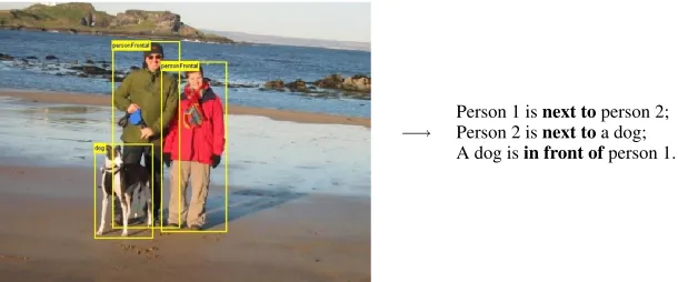
To illustrate the specific task we address, Fig-ure 1 shows an image from the VOC’08 data set (Everingham et al., 2010) complete with the origi-nal annotations, alongside the kind of descriptions we aim to generate: each describes the spatial re-lationship between two of the objects in the image in simple terms focused around a preposition.
Over the following sections, we describe the data we used, with a particular focus on the set of prepositions used in the annotations (Section 2), outline the learning methods we tested (Section 3), and report the experiments we performed and the results we obtained (Section 4).
2 Data
Our starting point is the data set we adapted pre-viously (Belz et al., 2015) from the VOC’08 data (Everingham et al., 2010) by additionally annotat-ing images with prepositions which describe the spatial relationships between the annotated objects in the image.
We previously used a set of 38 prepositions which were obtained in the following fashion: (a) the (complete) image descriptions collected by Rashtchian et al. (2010) for 1,000 VOC’08 (Ev-eringham et al., 2010) images (five for each im-age) were parsed with the Stanford Parser version 3.5.21 with the PCFG model, (b) the nmod:prep
prepositional modifier relations were extracted au-tomatically, and (c) the non-spatial ones were re-moved manually. While this provided a non-arbitrary way of selecting a set of prepositions for the annotation task, it contained a large number of synonyms and near-synonyms (e.g.in, within, in-side), which appeared to make the learning task harder (see also discussion in Section 4.2 below).
Using as a basis the frequencies and synonym sets we reported previously (Belz et al., 2015), we map this set of 38 prepositions to a reduced set, as follows. We delete from the annotations
1http://nlp.stanford.edu/software/lex-parser.shtml
Person 1 isnext toperson 2;
[image:2.612.113.418.60.187.2]−→ Person 2 isnext toa dog; A dog isin front ofperson 1.
Figure 1: Image from VOC’08 with original annotations (left), and the kind of descriptions of spatial relationships we aim to generate automatically.
all those prepositions that were used five times or fewer by the annotators, leaving a set of 24 prepo-sitions; next, for each synonym set, we retain only the single preposition most frequently used by the annotators, and overwrite the other members of the set with it, yielding a final set of 16 prepositions. In the following sections, we refer to the data set with the larger number of prepositions as DS-38, and the data set with the smaller number as DS-16. All results reported for DS-16 in the present paper were obtained by training models directly on this new data set.
3 Learning Methods
We use a total of four different methods: a rule-based method and a Naive Bayes model that allow direct comparison to previous work, and two new methods, namely a support vector machine (SVM) model and a decision-tree (DT) model. The latter three methods all use the feature set described in Section 4.4 below.
Rule-based method (Elliot et al.): We use the implementation of Elliot et al.’s method we created previously (Belz et al., 2015) where handcrafted rules map a set of geometric features to the eight prepositions used by Elliot et al. (2014, p. 13).
Naive Bayes Model: We use a Naive Bayes model as in our previous work (Belz et al., 2015) which maps a set of nine handcrafted visual (in-cluding geometric) and verbal features to our set of 16 prepositions (for details of all see Section 4.4). The visual features include various measurements of object bounding box sizes, and overlap and dis-tance between bounding boxes, while the object labels provide the language features. The model uses the language features for defining the prior
model and the visual features for defining the like-lihood model.
SVM Model: Using the same features, we trained a multi-class SVM model employing one-versus-one classification.2 This involves
train-ing k(k−1)/2pairs of binary preposition clas-sifiers for a multi-class prediction task involving kprepositions. The SVM model was trained with an RBF kernel, characterised by a coefficient of 1/(|features|)and set to generate the probability estimates for all classes.
Decision-Tree Model: Again using the same features, we created a multi-class decision-tree model2 with a maximum tree depth of 4for the DS-16 data set, and5for the DS-38 data set (from training and validation error plots). The model generates the probability estimates for each class.
4 Experiments
The training data contains a separate training in-stance (Objs, Objo, p)for each prepositionp
se-lected by human annotators for the template ‘The Objs isptheObjo’ (e.g.the dog is in front of the
person) accompanied by an image in which (just) ObjsandObjoare surrounded by bounding boxes.
All models are trained and tested with leave-one-out cross-validation.
4.1 Evaluation methods
To compare results in this paper, we use the same variants of the basic Accuracy method as in our previous work (Belz et al., 2015). One dimension along which the variants differ is whether or not synonyms are allowed to substitute for each other. In those variants in which synonyms are allowed to
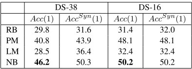
DS-38 DS-16
Acc(1) AccSyn(1) Acc(1) AccSyn(1)
RB 29.8 31.6 31.4 32.0
PM 40.8 43.9 48.1 48.1
LM 28.5 36.4 32.4 32.4
[image:3.612.99.296.58.129.2]NB 46.2 50.3 50.2 50.2
Table 1: Acc(1)andAccSyn(1)for the data with
the larger (DS-38) and smaller (DS-16) preposi-tion sets, and for the rule-based model (RB), the Naive Bayes model (NB), and the two component models of the NB model (PM and LM).
substitute for each other (AccSyn), a system output
is considered correct as long as it is in the same synonym set as the target (human-selected) output. Those variants which do not take synonyms into account are referred to simply asAcc.
The second dimension along which Accuracy variants differ is output rank. Different variants (denotedAcc(n)andAccSyn(n)) return Accuracy
rates for the topnoutputs, wheren = 1...4, pro-duced by systems, such that a system output is considered correct as long as the target (human-selected) output is among the top noutputs pro-duced by the system.
4.2 Comparing different preposition sets
The indication from the evaluation results reported we previously (Belz et al., 2015) was that the pres-ence of sets of synonymous prepositions in the data was adversely affecting the learning process. Note that while theevaluationsin that work took synonyms into account, thetraining phasedid not. AccSyn results in the previous work were higher
than Accresults for all methods investigated, by between 2 and 6 percentage points. This indicated that higher Accuracy rates could be achieved by reducing the number of synonymous prepositions. We tested this hypothesis in our first set of exper-iments, reported in this section, where we directly replicate the previous experiments, but training on our new annotations which eliminate synonyms.
Table 1 has direct comparisons of the results for the two methods tested in previous work (RB = rule-based model; NB = Naive Bayes model), for the original data set with 38 prepositions (DS-38) and the new version with 16 (DS-16). Note that as in the previous work the two component parts of the Naive Bayes model are also tested separately (PM = prior model; LM = likelihood model).
As expected, the main results (Acc(1)figures)
are higher for DS-16 for all four models. The pact is greatest for the PM model, which is im-proved by just over 7 percentage points. The head-line results (highlighted in bold in the table) show that the best model (NB) improves by 4 percent-age points through the removal of synonyms from the training set, almost the exact extent predicted by theAccSynresults for DS-38.
4.3 Comparing different models
We tested the two previous methods (RB and NB) as well as two new models (SVM and DT) on both the DS-38 and the DS-16 data sets (for descrip-tions of the four models see Section 3). For the first set of experiments, we tested the four models on the two data sets using the same nine features used previously (experiments for different feature sets are reported in the following section).
The results are shown in Table 2. TheAccand AccSynnumbers show that the Naive Bayes model
outperforms the rule-based baseline, the SVM and the decision tree under all conditions tested.
Looking at results for 38 compared to DS-16, we see that the SVM and DT models also ben-efit substantially from the removal of synonyms in the annotations; in fact the benefit is great-est for the SVM method (27 vs. 35.6). Informal examination of the SVM output also shows that this method is particularly sensitive to differences in preposition frequencies, tending to cluster the prepositions around the 7 or 8 highest-frequency prepositions.
4.4 Comparing different feature sets
The third aspect we investigated was the set of fea-tures being used in each method, again with a view to improving results. The results reported in previ-ous sections above were all obtained with the same set of nine features:
F0: Object labelLs.
F1: Object labelLo.
F2: Area of bounding box of Objs
nor-malised by image size.
F3: Area of bounding box of Objo
nor-malised by image size.
F4: Ratio of area ofObjs bounding box to
that ofObjo.
F5: Distance between bounding box cen-troids.
DS-38
Model n= 1 n= 2 Accn(1= 3..n) n= 4
RB 29.8 38.7 44.5 44.6
NB 46.2 60.6 69.9 77.6
SVM 27.0 47.0 56.2 65.2
DT 39.3 53.4 67.2 73.7
AccSyn(1..n)
n= 1 n= 2 n= 3 n= 4
RB 31.6 40.8 46.6 46.7
NB 50.3 63.9 72.2 80.0
SVM 29.8 52.6 63.5 69.7
DT 41.6 56.5 71.1 76.1
DS-16
Model n= 1 n= 2Acc(1..nn)= 3 n= 4
RB 31.4 41.3 46.5 46.7
NB 50.2 65.2 76.5 83.9
SVM 35.8 56.0 72.7 78.9
DT 42.8 59.8 73.1 81.8
AccSyn(1..n)
n= 1 n= 2 n= 3 n= 4
RB 32.0 41.6 46.5 46.7
NB 50.2 65.2 76.5 83.9
SVM 35.8 56.0 72.7 78.9
[image:4.612.135.483.59.185.2]DT 42.8 59.8 73.1 81.8
Table 2:AccandAccSynresults for all four models (leaving out component models) described in
Sec-tion 3, and the two data sets described in SecSec-tion 2.
F7: Distance between centroids divided by the approximated average width of the two bounding boxes.
F8: Position ofObjsrelative toObjo(N, E,
[image:4.612.317.512.235.361.2]S, W).
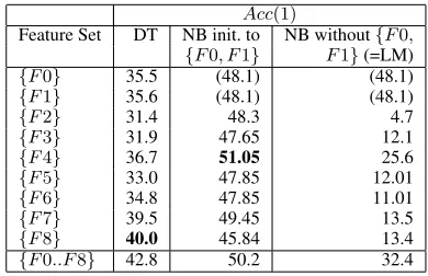
Table 3 shows Accuracy rates achieved using the same experimental set-up as in previous sections, but using just single features (where this is pos-sible3). The bottom row, for ease of reference,
shows the Accuracy achieved when using the com-plete set of 9 features.
The numbers show that the different features achieve varying Accuracy rates within the context of each of the two methods. For example, it is F7 that achieves the highest Accuracy on its own in the NB method, but F8 in the DT method. It is also noticeable that, for the NB model, F4 (ratio of bounding box sizes) on its own achieves a bet-ter result than all features combined.
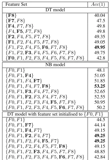
The above only tells us about individual fea-tures in isolation, so we also carried out greedy feature selection using theLASSOmethod, adding the best feature in each round (using our own im-plementation). The results are shown in Table 4, as applied to the DT model at the top, and the NB model in the middle. Note that because the two language features,F0andF1, constitute the (sep-arate) prior model component in the NB model (with the remaining features making up the like-lihood model), we cannot applyLASSOto the NB
model in quite the same way as for the DT model, instead initialising the feature set to {F0, F1}. For comparability, we also show results for doing the same for the DT model (lower third of Table 4).
3For the NB model, we report two columns of results, one
for the model initialised to F0 and F1, and the other for the NB model without F0 and F1, which makes it the LM model.
Acc(1)
Feature Set DT NB init. to NB without{F0,
{F0, F1} F1}(=LM)
{F0} 35.5 (48.1) (48.1)
{F1} 35.6 (48.1) (48.1)
{F2} 31.4 48.3 4.7
{F3} 31.9 47.65 12.1
{F4} 36.7 51.05 25.6
{F5} 33.0 47.85 12.01
{F6} 34.8 47.85 11.01
{F7} 39.5 49.45 13.5
{F8} 40.0 45.84 13.4
{F0..F8} 42.8 50.2 32.4
Table 3: Acc(1) for each feature individually (where possible), for the smaller (DS-16) number of prepositions, for the Decision Tree and Naive Bayes models (F0andF1are the language fea-tures, andF2..F8are the vision features).
Some commonalities emerge, e.g.F4, F7and F8 are high-performing features that tend to be selected early, whileF6tends to be selected late. In all three cases, greedy feature selection reveals a maximum (highlighted in bold) before the com-plete set of features is reached which outperforms results achieved with all features, by a margin of between 3 and just over 7 percentage points.
The highest Accuracy achieved (53.25) is lower than accuracy rates reported in other preposition prediction research (Ramisa et al., 2015); however that work used different datasets and results varied widely between them.
5 Discussion
from the annotations. Two new learning methods, SVMs and decision-trees, did not in themselves result in improved scores. Finally, a simple ap-proach to feature set optimisation, greedy LASSO
feature selection, further improved the best Accu-racy score from 50.2 to 53.25.
Not surprisingly, while feature set optimisation improves Acc(n) scores for n = 1, it has less effect on scores for other values of n. E.g., for the optimised NB model, the four scores forn = 1, n= 2, n = 3, andn = 4are 53.3, 66.7, 76.2, and 82.9, respectively, while for the non-optimised NB model, they are 50.2, 65.2, 76.5, and 83.9.
Out of those cases where the models do not get it right, they get it nearly right a lot of the time, as can be seen by comparing theAcc(n)scores for different values ofnin Table 2. In fact the margins between the Acc(1) scores (proportion of times the correct result was ranked top by a model), and the scores for other values of n (proportion of times the correct result was one of the top n selected by a model) are greater for the new im-proved results using DS-16, as can be verified by looking at the top left and top right quarters of Ta-ble 2. This may indicate that there is room for fur-ther improvement, using more data or ofur-ther learn-ing methods. Another avenue for investigation is human evaluation of the results which would re-veal how often the preposition selected by a model for a given pair of objects is in fact deemed correct by humans even though it happens to be not con-tained in the annotations for that image.
6 Conclusion
In this paper, we have investigated the effects of varying three different aspects of learning to gen-erate prepositions that describe the spatial rela-tionship between two objects in an image: the set of prepositions, the type of learning method, and the set of features. The investigations led to improvements in Accuracy results from 46.2 to 53.25. Among other findings we saw that the more useful features tended to be those that capture a property of the two objects together (such as the ratio between the sizes of their bounding boxes), and that the general usefulness of features depends on the model they are used in conjunction with.
References
Anja Belz, Adrian Muscat, Maxime Aberton, and Sami Benjelloun. 2015. Describing spatial relationships
Feature Set Acc(1)
DT model
{F8} 40.04
{F7, F8} 47.5
{F4, F7, F8} 49.8
{F4,F5, F7, F8} 49.8
{F2, F4, F5, F7, F8} 49.35
{F1, F2, F4, F5, F7, F8} 49.05
{F1, F2, F4, F5,F6, F7, F8} 49.95
{F1, F2,F3, F4, F5, F6, F7, F8} 49.75
{F0, F1, F2, F3, F4, F5, F6, F7, F8} 42.8 NB model
{F0, F1} 48.1
{F0, F1,F4} 51.05
{F0, F1, F4,F7} 51.85
{F0, F1, F4, F7,F8} 53.25
{F0, F1,F3, F4, F7, F8} 52.65
{F0, F1,F2, F3, F4, F7, F8} 52.55
{F0, F1, F2, F3, F4,F5, F7, F8} 50.95
{F0, F1, F2, F3, F4, F5,F6, F7, F8} 50.2 DT model with feature set initialised to{F0, F1}
{F0, F1} 44.5
{F0, F1,F7} 44.14
{F0, F1,F4, F7} 49.15
{F0, F1,F2, F4, F7} 49.25
{F0, F1, F2, F4,F5, F7} 49.25
{F0, F1, F2, F4, F5, F7,F8} 49.15
{F0, F1, F2,F3, F4, F5, F7, F8} 48.85
[image:5.612.319.509.57.335.2]{F0, F1, F2, F3, F4, F5,F6, F7, F8} 42.84
Table 4: Acc(1) figures when applying LASSO
greedy feature selection for DT and NB models, and for DT model withF0andF1fixed, for di-rect comparability with NB model.
between objects in images in English and French. In The 4th Workshop on Vision and Language (VL’15). Desmond Elliott. 2014. A Structured Representation of Images for Language Generation and Image Re-trieval. Ph.D. thesis, University of Edinburgh. Mark Everingham, Luc Van Gool, Christopher KI
Williams, John Winn, and Andrew Zisserman. 2010. The PASCAL Visual Object Classes (VOC) Challenge. International Journal of Computer Vi-sion, 88(2):303–338.
Arnau Ramisa, Josiah Wang, Ying Lu, Emmanuel Dellandrea, Francesc Moreno-Noguer, and Robert Gaizauskas. 2015. Combining geometric, tex-tual and visual features for predicting prepositions in image descriptions. InProceedings of the 2015 Conference on Empirical Methods in Natural Lan-guage Processing, pages 214–220, Lisbon, Portugal, September. Association for Computational Linguis-tics.