Estimation of Distribution Algorithm with Multivariate T Copulas for Multi Objective Optimization

Estimation of Distribution Algorithm with Multivariate

T

-Copulas for Multi-Objective Optimization

Ying Gao, Lingxi Peng, Fufang Li, Miao Liu, Xiao Hu

Department of Computer Science and Technology, Guangzhou University, Guangzhou, China Email: [email protected]

Received September 10, 2012; revised October 10, 2012; accepted October 18, 2012

ABSTRACT

Estimation of distribution algorithms are a class of evolutionary optimization algorithms based on probability distribu- tion model. In this article, a Pareto-based multi-objective estimation of distribution algorithm with multivariate T- copulas is proposed. The algorithm employs Pareto-based approach and multivariate T-copulas to construct probability distribution model. To estimate joint distribution of the selected solutions, the correlation matrix of T-copula is firstly estimated by estimating Kendall’s tau and using the relationship of Kendall’s tau and correlation matrix. After the cor- relation matrix is estimated, the degree of freedom of T-copula is estimated by using the maximum likelihood method. Afterwards, the Monte Carte simulation is used to generate new individuals. An archive with maximum capacity is used to maintain the non-dominated solutions. The Pareto optimal solutions are selected from the archive on the basis of the diversity of the solutions, and the crowding-distance measure is used for the diversity measurement. The archive gets updated with the inclusion of the non-dominated solutions from the combined population and current archive, and the archive which exceeds the maximum capacity is cut using the diversity consideration. The proposed algorithm is ap- plied to some well-known benchmark. The relative experimental results show that the algorithm has better performance and is effective.

Keywords: Estimation of Distribution Algorithm; Pareto-Based Approach; T-Copulas; Multi-Objective Optimization

1. Introduction

Optimization problems are widely encountered in various fields of science and technology. When an optimization problem involves only one objective function, the task of obtaining the optimal solution is called single objective optimization. When an optimization problem involves more than one objective function, the task of finding one or more optimum solutions is called multi-objective op- timization. Many real-world optimization problems in- volve multiple objectives. The fundamental difference between single-objective and multi-objective optimiza- tion lies in the cardinality of the optimal set. In problems with two or more conflicting objectives, there is no sin- gle optimum solution. There exist a number of solutions which are optimal. Such solutions are called Pareto-op- timal solutions. The solution to a multi-objective optimi- zation problem consists of a solution set with multiple solutions that may produce tradeoffs between different objectives. These solutions are called non-dominated so- lutions and the corresponding solution set is called the Pareto-front [1]. None of the solutions in the Pareto-front is best with respect to all objectives. In addition, no solu- tion in the Pareto-front is better than any other solution in

the front with respect to all objectives. Hence, without any additional problem-specific information about the priorities of various objectives, all the solutions in the Pareto-front are important. The main objective of multi- objective optimization is to find many such solutions which reflect the tradeoffs between the objectives. Multi- objective optimization algorithms, especially those based on evolutionary principles, have been widely used to solve problems with multiple objectives. In recent years, a considerable amount of interest has been shown in mul- ti-objective evolutionary algorithm (MOEA) and a num- ber of different MOEAs have been suggested, such as Strength Pareto Evolutionary Algorithm (SPEA2) [2], Non-dominated Sorting Genetic Algorithm (NSGA-II) [3], and Fast Pareto Genetic Algorithm (FastPGA) [4].

estimates and samples the probability distribution. A wide variety of EDAs using different techniques to esti- mate and sample the probability distribution have been proposed and are the subject of active research. Many EDAs use probabilistic graphical modeling techniques [6, 7] for this purpose. However, EDA using probabilistic graphical modeling techniques generally spend too much time on the learning about the probability distribution of the promising individuals. Copula [8,9] is a recently de- veloped mathematical theory and a power tool for multi- variate probability analysis. According to copula theory, a joint probability distribution can be decomposed into n marginal probability distributions and a copula function. So, the joint probability distribution of multivariate can be constructed utilizing a copula function and the mar- ginal probability distributions of every variable. Copulas have be applied to constitute the probabilistic model in the conventional EDAs [10,11]. It is simpler and easier to model the probability distribution compared with other methods in EDAs.

In this paper, EDA is extended to multi-objective op- timization problems by using a Pareto-based approach and T-copulas. The extended multi-objective EDA em- ploys multivariate T-copulas to construct probability dis- tribution model. T-copula parameters are firstly estimated, thus, joint distribution is estimated by estimating Kend- all’s tau and using the relationship of Kendall’s tau and correlation matrix. After the correlation matrix is esti- mated, the degree of freedom of T-copula is estimated by using the maximum likelihood method. Afterwards, the Monte Carte simulation is used to generate new indivi- duals. An archive with maximum capacity is used to ma- intain the non-dominated solutions. The Pareto optimal solutions are selected from the archive on the basis of the diversity of the solutions, and the crowding-distance measure is used for the diversity measurement. The ar- chive gets updated with the inclusion of the non-domi- nated solutions from the combined population and cur- rent archive, and the archive which exceeds the maxi- mum capacity is cut using the diversity consideration. The proposed algorithm is applied to some well-known benchmark. The relative experimental results show that the algorithm has better performance and is effective.

2. Multi-objective Optimization Problems

The general multi-objective optimization problem can be defined as follows:

 



1

  

2

minF x  f x ,f x



, , fk

 

x



1, 2, ,

s.t. gi

 

0, i  m 1, 2, ,

h  i  p



n X

 

x (1)

 

0,

i x



x x, , ,x



x 

(2) where is an n-dimensional deci-

sion variable vector and X is the decision variable space. The constrains given by (1) and (2) define the feasible region Ω and any point in Ω defines a feasible solution.

1 2



,



M y y F x x  

 

F x

 is referred to as objective space. The k components of the vector are the criteria to be considered. The constrains gi

 

x and

 

h x



i represent the restrictions imposed on the decision

variables.

When there are several objective functions, the con- cept of optimum changes, because in multi-objective op- timization problems the purpose is to find “trade-off so- lutions rather than a single solution. The concept of op- timum commonly adopted in multi-objective optimiza- tion is Pareto optimality. Pareto optimality is defined as:

A point x   is Pareto optimal if   x and



1, 2, ,k



  either:

 



I i I f fi





  x  x

i I i

and, there is at least one  such that f

 

x  f



x





x x

i i

This definition says that is Pareto optimal if there exists no feasible vector which would decrease some criteria without causing a simultaneous increase in at least one other criterion. Other important definitions as- sociated with Pareto optimality are Pareto dominance.



x x1, , ,2 xn





x  is said to dominate A vector



y y1, , ,2 yn





y  , denoted by x y



1, 2, ,



i k

   _{i i}

, if and only if x is partially less than y, i.e., x  y and, at least for one i, xi yi.

For a given multi-objective problem , the Pareto

optimal set

 

F x

P is defined as:



 

 



P x    x F x F x

 

F x

, P

For a given multi-objective problem and Pareto optimal set  the Pareto front PF is defined as:

 

   

 





1 , 2 , , k





PF_{ F x } f _x f _{x } f _{x x}P

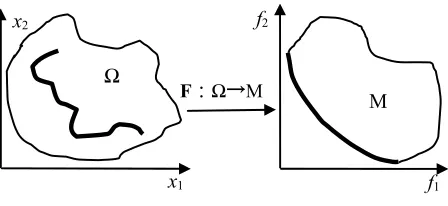
P The set of all Pareto optimal solutions in the feasible region Ω is called Pareto optimal set and the correspond- ing set of objective vector is called Pareto optimal front. The illustrative example of a multi-objective minimiza- tion problem with two objectives, f1 and f2, that are plot-

ted in the objective space M mapped from the feasible region Ω is shown in Figure 1. The bold curve in the feasible region Ω indicates the Pareto optimal set _.

The bold curve in the objective space M indicates the Pa- reto front _PF_.

3. Multivariate

T

-Copulas

[image:3.595.62.286.86.189.2]

F：Ω→M f2 f1 x2 x1 Ω M

Figure 1. The illustrative example.

tion. The major issues in estimation of distribution algo- rithms are how to build a probability distribution model and how to sample the new individuals according to the probability distribution model.

The theory of copulas is known to provide a useful tool for modelling dependence in many applications. Co- pulas have attracted significant attention in the recent li- terature for modeling probability distribution of multi- variate observations. An important feature of copulas is that they enable us to specify the univariate marginal dis- tributions and their joint behavior separately. Archime- dean Copula and Gaussian Copula have be applied to constitute the probabilistic model in EDAs [10,11].

The copula theory is briefly introduced in the follow- ing, the details can be found in [8,9].

An n-dimensional copula is a multivariate C.D.F., C, with uniformly distributed margins on [0, 1] (U(0,1)) and the following properties:

1) C: [0, 1]n_{→ [0, 1];}

2) C is grounded and n-increasing; 3) C has margins Ci which satisfy

for all

 



1, ,1,

i u

C C  u,1, ,1



u u

 

0,1

1, , n . It is obvious, from the above definition, that if F  F

 



, , F x



1, , i  n

, ,

are univariate distribution functions,

is a multivariate C.D.F. with

margins ₁ , since , , is a

uniform random variable. Copula functions are a useful tool to construct and simulate multivariate distributions.

 

1 1

C F x n n

, , _n

F  F U_i F_i

 

X_i

The following theorem is known as Sklar’s Theorem. It is the most important theorem regarding to copula functions since it is used in many practical applications.

Theorem:LetFbeann-dimensionalC.D.F. withcon- tinuous margins F₁ F_n. Then F has the following unique copula representation (canonical decomposi- tion):



1, ,







1

 

 



F x  xn C F x₁ , , F xn n

1, , n

(3) The theorem of Sklar is very important, because it provides a way to analyse the dependence structure of multivariate distributions without studying marginals dis- tributions. From Sklar’s theorem we see that, for con- tinuous multivariate distribution functions, the univariate margins and the multivariate dependence structure can be

separated. The dependence structure can be represented by an adequate copula function. Moreover, the following corollary is attained from (3).

Corollary: Let F be an n-dimensional C.D.F. with continuous margins F  F and copula C (satisfying (3)). Then, for any u



u1, , un



in [0,1]n:







1

 

1

 



1, , n 1 1 , , n n

 



C u  u F F u  F u

1

(4)



where Fi is the generalized inverse of Fi.

The T-copula can be thought of as representing the dependence structure implicit in a multivariate T-distri- bution. For a symmetric and positive definite matrix

 

r ,i 1, 2, , ,n j 1, 2, ,n

  

R  

T

,

i j with unit diagonal

entries, let R,v denote the standardized multivariate Student’s T-distribution with correlation matrix R and

degrees of freedom: 1 v





 

  1 1 2 , 1 2 2 T 1 1 2 , , π 2 1

1 d d

n

y y

R v n

n

v n

n

v n

T y y

v _v x x v                  _{ }    _{ }  





R

x R x

 



(5)

The multivariate T-copula (MTC) is defined as:







1

 

1

 



1, , , ; ,2 n ,v v 1 , , v n

C u u u v _T T u T u

R

R

 

1 T where v

 _{is the inverse of the univariate Student’s t}

cumulative distribution function with v degrees of free- dom.

The corresponding density is





 





 

1 2 1 2

2 T 1

1 2 2

1

1 2 2

, , , ; , 1 2 2 1 1 1 n n v n v n j j

v n v

c u u u v

v v v v               _{ } _{  }  _   _         _{  }_{ }       _       



R R

ω R ω





_{ , , ,}



T_{;  T}1

 

_{u ,j 1, ,n}

    

ω

(6)

with _{1 2 n j v j} .

A number of recent papers have shown that the em- pirical fit of the T-copula is generally superior to that of the so-called Gaussian copula, the dependence structure of the multivariate normal distribution. One reason for this is the ability of the T-copula to capture better the phenomenon of dependent extreme values. In the paper, we use T-copulas to model probability distribution in multi-objective estimation of distribution algorithm.

4. Multi-Objective EDA with

T

-Copulas

ing single objective optimization problems. However, the original scheme has to be modified for solving multi- objective optimization problems. As we saw in Section II, the solution set of a problem with multiple objectives does not consist of a single solution. Instead, in multi- objective optimization, we aim to find Pareto optimal set. Besides using multivariate T-copulas for constructing pro- bability distribution model in the multi-objective EDA, we have used an archive with maximum capacity to ma- intain the non-dominated solutions and the crowding- distance measure for the diversity measurement. The Pa- reto optimal solutions are selected from the archive on the basis of the diversity of the solutions. The archive gets updated with the inclusion of the non-dominated so- lutions from the combined population and current archive, and the archive which exceeds the maximum capacity is cut using the diversity consideration. The algorithm steps of multi-objective EDA with T-copulas for solving multi- objective optimization problems are as follows:

t=0, initialize a population

S(0)Initialization ()

inated(S(0))

Sample()



(S(t) S (t)) 

(t 1) A(t))  ;

Evaluate(S(0))

A(0)Non_Dom

WHILE t < T DO

Estimate_Marginals_Distribution(); Estimate_Correlation_Matrix(); Estimate_Degrees_Freedom();

S ( )t

S(t

;

1) Selection

  Evaluate(S(t+1))

A(t 1) Non_Dominated(S

IF A(t1) M THEN Cut_Archive(A( 1))t t 1

t  END WHILE

Output obtained Pareto optimal front

The function initialization() is used to initialize a popu- lation S(0) with size N. The initial population S(0) is chosen randomly and should uniformly cover the entire solution space based on the consideration of the require- ment of population diversity. The function Evaluate() is used to evaluate each individual in population. The ar- chive A(0) has been initialized to contain the non-domi- nated solutions from S(0). The function Non_Domina() returns the non-dominated solutions from a population.

The function Estimate_Marginals_Distribution() is used to estimate the marginals distribution from population. The function Estimate_Correlation_Matrix() is used to estimate the correlation matrix R in T-copulas.

A simple method [9] based on Kendall’s tau is applied for estimating the correlation matrix R. The method con- sists of constructing an empirical estimate of Kendall’s

tau for each bivariate margin of the copula and then us- ing relationship (7)





 

,

2

, arcsin

π

k m rk m

 X X 



k, m





(7)

To infer an estimate of the relevant element of R. More specifically we estimate X X by calculat- ing the standard sample c coefficient









1







ˆ ,

2 _sign

1 k m

i,k j,k i,m j,m i j n

X X X X

n n 

  

 

 _   _





X X

, , ,

(8)

From the original data vectors X₁ X₂ XN, and write the jth component of the ith vector as Xi j, ; this

yields an unbiased and consistent. An estimator of rk m, is then given by ,





π

ˆ sin ˆ ,

2

k m k m

r  _  _

 X X 

R

,

ˆ_{k m} r

. In order to obtain an estimator of the entire matrix we can col- lect all pairwise estimates and then construct the estimator





π

ˆ _{sin ˆ , , 1, , , 1, ,}

2 k m k N m N

  

_{  }  

 

 

R X X   (9)

Then, The function Estimate_Degrees_Freedom() is used to estimate the degrees of freedom v by maximum likelihood method.

The function Sample() is used to generate offspring population S t

 

by sampling a T-copula function TR,v with correlation matrix and v degrees of freedom can be generated as follows [9].

R

R

T

1) Find the Cholesky decomposition of , so that

AA R, with A lower triangular;

2) Generate a sample of n independent random vari- ables Z 



z z, , , z



Tfrom N(0, 1);

2

v

1 2 n

3) Generate an independent random variables s with Z from  distribution;

v 4) Set Y AZ,

s 

W Y





T

1, 2, , n

w w w



W 



1, , ,2



T n

y y y

 

with

and Y ;

 

j , 1, , u T w j  n 5) Set j v

6) Return

;







1

 

1

 

1

 



1, , ,2 n 1 1 , 2 2 , , n n

x x x F u F u F u

 

X  

 

S t

. The function Selection() is used to evaluate each indi- vidual in the current population and the offspring population S t

 

and carry out the non-dominated sort- ing and ranking selection, developed by Deb etal. in [3] to select non-dominated individuals to constitute the next generation population S t



1



.



1



S t

 

solutions from the next generation population 

and the archive xi 0,1

 





 

A t

1 1

. If the size of the archive exceeds the maximum capacity M, it is cut using the diversity consideration. The function Cut_Archive() is used to cut the archive.

5. Simulation Results

In order to test efficiency of the Pareto-based multi-ob- jective estimation of distribution algorithm with T-copu- las, the performance of the proposed algorithm is com- pared with that of some multi-objective optimization al- gorithms. The following some well-known benchmark functions [12] have been used to test.

1) ZDT1:

 

f x x

 

 



x g

 

x



2 1 1

f x g x  xi

 

0,1





 



2 i



1

g x D

1 1

1 9 _iD_

 



x

2) ZDT2:

 

f x

 

x

 

 





2



2



1 x g1 x



f x g x  xi 0,1











 

2 1

D i

g x D

1 1

1 9



_i

 

x

3) ZDT3:

 

f x x

 

 

_{ }

1

_{  }

1



1

1 x x sin 10π

2

f g x

g g

 

 _   _

 

x x

x x



0,1



i

x 

 

1 9



2





1



D i i

g x  



_ x D

1 1 4) ZDT4:

 

f x x

 

 



 



2 1 1

f x g x  x g x

 





1 0,

2,



1 , i

x  x 

,

i  D

5,5 ,



 







2







2

1 10 1 D_{i i} 10 cos 4π_i

g x   D 



_ x  x

5) ZDT6:

 





6





1 1 exp 4 1 sin 6π1

f    x x

 

   

x

 







2



2 1 1

f x g x  f x g x





0.25

2

1 9 Di i 1

g x  



_ x D

The two common metrics used to compare are con- vergence metric γ and divergence metric Δ. For these metrics we need to know the true Pareto front for a prob- lem. In our experiments we use 1000 uniformly spaced Pareto optimal solutions as the approximation of the true Pareto front. A brief introduction of these metrics is given here:

Convergence metric γwas proposed by Deb et al.[3], measures the distance between the obtained non-domi- nated front NF and optimal Pareto front PF. Mathemati-cally, it may be defined as:

1

N

i i

d

N







γ

d

(10)

where N is the number of non-dominated solutions found by the algorithm being analyzed and i is the minimum Euclidean distance (measured in the objective space) between the ith solution of NF and the solutions in PF.

Diversity metric Δ was proposed by Deb et al. [3]. It measures the extent of spread achieved among the ob- tained solutions and is defined as:





1

1

1 s

f i i

i

f i

d d d d

d d s d

 

  



  



Δ where

1

1

1 s

i i

d d

s

 

 



(11)

where s is the number of members in the set of non- dominated solution found so far, and the parameter df

d

and i are the Euclidean distances between the extreme solutions and the boundary solutions of the obtained non-dominated set. The parameter d is the average of all distances d ii



1, , s1



, assuming that there are s

solutions on the best non-dominated front. The smaller the value of these metrics is, the better the performance of the algorithm is. The initial population was generated from a uniform distribution in the ranges specified below. Population size N = 80. All experiments were repeated for 30 runs. The maximum number of iterations is set to 1000 in each running.

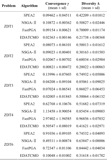
Table 1 listed the mean and standard deviation(sd) values of convergence metric γ and diversity metric Δ

[image:6.595.59.286.113.455.2]

Table 1. Mean and sd of the convergence and diversity met- rics for Benchmark functions.

Problem Algorithm Convergence _{(mean ± sd)} γ Diversity _{(mean ± sd)} Δ

SPEA2 0.09462 ± 0.04511 0.42209 ± 0.01012

NSGA-Ⅱ 0.10872 ± 0.00362 0.50827 ± 0.02446

FastPGA 0.09154 ± 0.00621 0.70009 ± 0.01174 ZDT1

EDATCMO 0.02363 ± 0.00146 0.21738 ± 0.00368

SPEA2 0.08073 ± 0.06101 0.50013 ± 0.01612

NSGA-Ⅱ 0.09023 ± 0.00401 0.30163 ± 0.01503

FastPGA 0.02067 ± 0.00702 0.60034 ± 0.02984 ZDT2

EDATCMO 0.00821 ± 0.00472 0.20022 ± 0.00863

SPEA2 0.13996 ± 0.07603 0.74932 ± 0.05006

NSGA-Ⅱ 0.04208 ± 0.09104 0.85061 ± 0.09025

FastPGA 0.07024 ± 0.06541 0.86027 ± 0.06453 ZDT3

EDATCMO 0.02005 ± 0.01843 0.50064 ± 0.06132

SPEA2 0.62768 ± 0.10676 0.51682 ± 0.07319

NSGA-Ⅱ 1.13458 ± 0.90054 0.85454 ± 0.09003

FastPGA 2.97402 ± 1.94585 0.96856 ± 0.07032 ZDT4

EDATCMO 0.50547 ± 0.08019 0.41621 ± 0.02971

SPEA2 0.91036 ± 0.09105 0.74532 ± 0.04093

NSGA-Ⅱ 0.49311 ± 0.00874 0.63847 ± 0.08006

FastPGA 0.72347 ± 0.01106 0.84442 ± 0.04034 ZDT6

EDATCMO 0.10048 ± 0.01002 0.31618 ± 0.01782

than those obtained by using SPEA2, NSGA-II, FastPGA. It indicates that EDATCMO outperforms SPEA2, NS- GA-II and FastPGA algorithms on the benchmark func- tions in both aspects of convergence and distribution of solutions.

6. Conclusion

We proposed a multi-objective estimation of distribution algorithm using T-copulas and Pareto-based approach. The proposed algorithm employs the multivariate T- copulas to construct probability distribution model, and the new individuals are generated according to the prob- ability distribution model. An archive is used to maintain the non-dominated solutions. The Pareto optimal solu- tions are selected from the archive. The archive gets up- dated with the inclusion of the non-dominated solutions from the combined population and current archive. The algorithm is applied to some well-known benchmarks. The results show that the algorithm has better perform- ance than SPEA2 [2], NSGA-II [3], FastPGA [4] on the multi-objective benchmark functions ZDT1, ZDT2, ZDT3, ZDT4 and ZDT6.

7. Acknowledgements

This work is supported by the Scientific and Technolo- gical Innovation Projects of Department of Education of Guangdong Province, P.R.C. Grant No. 2012KJCX0082 and Science and Technology Projects of Guangdong Pro- vince, P.R.C. under Grant No. 2011B090400623, Guang- zhou Science and Technology Pprojects under Grant No. 12C42011563, 11A11020499.

REFERENCES

[1] C. A. Coello, “A Comprehensive Survey of Evolution- ary-Based Multi-objective Optimization Techniques,” In- ternational Journal of Knowledge and Information Sys- tems, Vol. 1, No. 3, 1999, pp. 269-308.

[2] E. Zitzler, M. Laumanns and L. Thiele, “SPEA2: Im- proving the Strength Pareto Evolutionary Algorithm for Multi-Objective Optimization,” Proceedings of the EU- ROGEN Conference, Lake Como, 2001, pp. 95-100. [3] K. Deb, S. Agrawal, A. Pratap and T. Meyarivan, “A Fast

and Elitist Multi-Objective Genetic Algorithm: NSGA-II,” IEEE Transactions on Evolutionary Computation, Vol. 6, No. 2, 2002, pp. 182-197. doi:10.1109/4235.996017 [4] H. Eskandari, C. D. Geiger and G. B. Lamont, “FastPGA:

A Dynamic Population Sizing Approach for Solving Ex- pensive Multi-Objective Optimization Problems,” In: Evo- lutionary Multi-objective Optimization Conference EMO, Springer-Verlag, Berlin, Heidelberg, 2007, pp. 141-155. [5] P. Larranaga and J. A. Lozano, “Estimation of Distribu-

tion Algorithms: A New Tool for Evolutionary Computa- tion,” Kluwer Academic Publishers, Dordrecht, 2002. doi:10.1007/978-1-4615-1539-5

[6] S. Shakya, “DEUM: A Framework for an Estimation of Distribution Algorithm Based on Markov Random Fields,” Ph.D. thesis, The Robert Gordon University, Aberdeen, 2006.

[7] S. Shakya and J. McCall, “Optimisation by Estimation of Distribution with DEUM Framework Based on Markov Random Fields,” International Journal of Automation and Computing, Vol. 4, No. 3, 2007, pp. 262-272. doi:10.1007/s11633-007-0262-6

[8] R. B. Nelsen, “An Introduction to Copula,” Springer-Ver- lag, New York, 1998.

[9] U. Cherubini, E. Luciano and W. Vecchiato, “Copula Me- thods in Finance,” John Wiley & Sons Ltd., Chichester, 2004.

[10] Y. Gao, “Multivariate Estimation of Distribution Algo- rithm with Laplace Transform Archimedean Copula,” IEEE International Conference on Information Engineer- ing and Computer Science, Vol. 1, 2009, pp. 273-277. [11] Y. Gao, X. Hu, H. L. Liu, F. F. Li and L. X. Peng, “Op-

[12] E. Zitzler, K. Deb and L. Thiele, “Comparison of Multi- Objective Evolutionary Algorithms: Empirical Results,”