Towards Automatic Description of Knowledge Components

Towards Automatic Description of Knowledge Components

Cyril Goutte National Research Council

1200 Montreal Rd. Ottawa, ON K1A0R6

[email protected]

Guillaume Durand National Research Council

100 des Aboiteaux St. Moncton, NB E1A7R1

[email protected]

Serge L´eger National Research Council

100 des Aboiteaux St. Moncton, NB E1A7R1

[email protected]

Abstract

A key aspect of cognitive diagnostic models is the specification of the Q-matrix associat-ing the items and some underlyassociat-ing student attributes. In many data-driven approaches, test items are mapped to the underlying, la-tent knowledge components (KC) based on observed student performance, and with little or no input from human experts. As a result, these latent skills typically focus on model-ing the data accurately, but may be hard to describe and interpret. In this paper, we fo-cus on the problem of describing these knowl-edge components. Using a simple probabilis-tic model, we extract, from the text of the test items, some keywords that are most rel-evant to each KC. On a small dataset from the PSLC datashop, we show that this is surpris-ingly effective, retrieving unknown skill labels in close to 50% of cases. We also show that our method clearly outperforms typical base-lines in specificity and diversity.

1 Introduction

Recent years have seen significant advances in auto-matically identifying latent attributes useful for cog-nitive diagnostic assessment. For example, the Q-matrix (Tatsuoka, 1983) associates test items with skills of students taking the test. Data-driven meth-ods were introduced to automatically identify latent

knowledge components(KCs) and map them to test items, based on observed student performance, cf. Barnes (2005) and Section 2 below.

A crucial issue with these automatic methods is that latent skills optimize some well defined

objec-tive function, but may be hard to describe and in-terpret. Even for manually-designed Q-matrices, knowledge components may not be described in detail by the designer. In that situation, a data-generated description can provide useful informa-tion. In this short paper, we show how to extract keywords relevant to each KC, from the textual con-tent corresponding to each item. We build a simple probabilistic model, with which we score possible keywords. This proves surprisingly effective on a small dataset obtained from the PSLC datashop.

After a quick overview of the automatic extrac-tion of latent attributes in Secextrac-tion 2, we describe our keyword extraction procedure in Section 3. The data is introduced in Section 4, and we present our exper-imental results and analysis in Section 5.

2 Extraction of Knowledge Component Models

The Rule Space model (Tatsuoka, 1983; Tatsuoka, 1995) was introduced to statistically classify stu-dent’s item responses into a set of ideal response patterns associated with different cognitive skills. A major assumption of Rule Space is that students only need to master specific skills in order to successfully complete items. Using the Rule Space model for cognitive diagnostics assessment requires experts to build and reduce an incidence or Q matrix encoding the combination of skills, a.k.a. attributes, needed for completing items (Birenbaum et al., 1992) and generating ideal item responses based on the duced Q matrix (Gierl et al., 2000). The ideal re-sponse patterns can then be used to analyze student response patterns.

The requirement for extensive expert effort in the traditional Q matrix design has motivated attempts to discover the Q matrix from observed response patterns, in effect reverse engineering the design process. Barnes (2005) proposed a multi-start hill-climbing method to create the Q-matrix, but experi-mented only on limited number of skills. Desmarais et al. (2011; 2014) refined expert Q matrices using matrix factorization, Although this proved useful to automatically improve expert designed Q-matrices, non-negative matrix factorization is sensitive to ini-tialization and prone to local minima. Sun et al. (2014) generated binary Q-matrices using an alter-nate recursive method that automatically estimates the number of latent attributes, yielding high ma-trix coverage rates. Others (Liu et al., 2012; Chen et al., 2014) estimate the Q-matrix under the setting of well known psychometric models that integrate guess and slip parameters to model the variation be-tween ideal and observed response patterns. They formulate Q-matrix extraction as a latent variable selection problem solved by regularized maximum likelihood, but require to know the number of latent attributes. Finally, Sparse Factor Analysis (Lan et al., 2014) was recently introduced to address data sparsity in a flexible probabilistic model. They re-quire setting the number of attributes and rely on user-generated tags to facilitate the interpretability of estimated factors.

These approaches to the automatic extraction of a Q-matrix address the problem from various angles and an extensive comparison of their respective per-formance is still required. However, none of these techniques address the problem of providing a tex-tual description of the discovered attributes. This makes them hard to interpret and understand, and may limit their practical usability.

3 Probabilistic Keyword Extraction

We focus on the textual content associated with each item in order to identify the salient terms as key-words. Textual content associated with an item may be for example the body of the question, optional hints or the text contained in the answers (Figure 1). For each itemi, we denote bydiits textual content (e.g. body text in Figure 1). We also assume a bi-nary mapping of items toK skillsck,k = 1. . . K.

Skills are typically latent skills obtained automati-cally (unsupervised) from data. They may also be defined by a manually designed Q-matrix for which skill descriptions are unknown. In analogy with text categorization, textual content is a documentdiand each skill is a class (or cluster)ck. Our goal is to identify keywords from the documents that describe the classes.

For each KCck, we estimate a unigram language model based on all textdi associated with that KC. This is essentially building a Naive Bayes classifier (McCallum and Nigam, 1998), estimating relative word frequencies in each KC:

P(w|ck) = P

i,di∈cknwi

P

i,di∈ck|di|

, ∀k∈ {1. . . K}, (1)

wherenwi is the number of occurrences of wordw in documentdi, and|di|is the length (in words) of document|di|. In some models such as Naive Bayes, it is essential to smooth the probability estimates (1) appropriately. However more advanced multinomial mixture models (Gaussier et al., 2002), or for the purpose of this paper, smoothing has little impact. Conditional probability estimates (1) may be seen as the profile ofck. Important words to describe a KCc∈ {c1, . . . cK}have significantly higher prob-ability incthan in other KCs. One metric to evalu-ate how two distributions differ is the (symmetrized) Kullback-Leibler divergence:

KL(c, /c) =X

w (P(w|c)−P(w|/c)) log

P(w|c)

P(w|/c)

| {z }

k(w)

,

(2) where/cmeans all KCs exceptc, andP(w|/c)is esti-mated similarly to Eq. 1,P(w|/c)∝P_i,di6∈cnwi.

Note that Eq. (2) is an additive sum of posi-tive, word-specific contributions k(w). Large con-tributions come from significant differences either way between the profile of a KC,P(w|c), and the average profile of all other KCs, P(w|/c). As we want to focus on keywords that have significantly

higherprobability for that KC, and diregard words that have higher probabilityoutside, we will use a signed score:

Figure 1: Test item body text, hints and responses.

body hint response Total # tokens 31,132 11,505 41,207 83,844

Table 1: Dataset statistics, (# tokens).

where thelogensures that the score is positive if and only ifP(w|c)> P(w|/c).

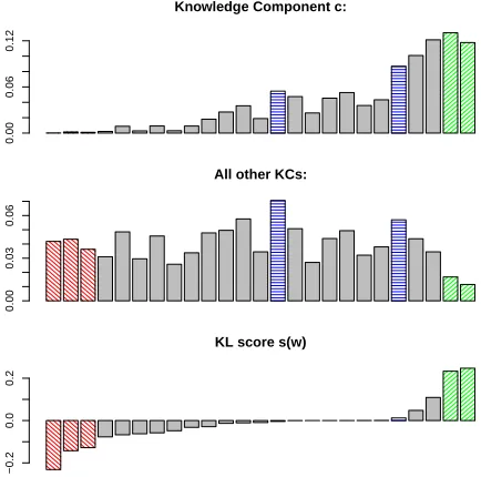
Figure 2 illustrates this graphically. Some words (blue horizontal shading) have high probability inc (top) but also outside (middle), hences(w)close to zero (bottom): they are not specific enough. The most important keywords (green upward shading, right) are more frequent inc than outside, hence a large score. Some words (red downward shading, left) are less frequent incthan outside: they do con-tribute to the KL divergence, but are atypical in c. They receive a negative score.

4 Data

In order to test and illustrate our method, we focus on a dataset from the PSLC datashop (Koedinger et al., 2010). We used theOLI C@CM v2.5 - Fall 2013, Mini 1.1 _{This OLI dataset tests proficiency with the} CMU computing infrastructure. It is especially well suited for our study because the full text of the items (cf. Fig. 1) is available in HTML format and can be easily extracted. Other datasets only include screen-shots of the item, making text extraction more chal-lenging.

There are 912 unique steps in that dataset, and less than 84K tokens of text (Table 1), making it very

1_{https://pslcdatashop.web.cmu.edu/DatasetInfo?datasetId=827}

Knowledge Component c:

0.00

0.06

0.12

All other KCs:

0.00

0.03

0.06

KL score s(w)

−0.2

0.0

0.2

Figure 2: KL score illustration: KC profile (top), profile for all other KCs (middle) and scores (bottom).

small by NLP standards. We picked two KC models included in PSLC for that dataset. ThenoSAmodel has 108 distinct KCs with minimally descriptive la-bels (e.g. “vpn”), assigning between 1 and 52 items to each KC. The C75 model is fully unsupervised and has the best BIC reported in PSLC. It contains 44 unique KCs simply labelledCxx, withxxbetween -1 and 91. It assigns 5 to 78 items per KC. In both models there are 823 items with at least 1 KC as-signed.

We use a standard text preprocessing chain. All text (body, hint and responses) in the dataset is to-kenized and lowercased, and we remove all tokens appearing in an in-house stoplist, as well as tokens not containing at least one alphabetical character.

5 Experimental Results

From the preprocessed data, we estimate all KC pro-files using Eq. (1), on different data sources:

1. Only the body of the question (“body”), 2. Body plus hints (“b+h”),

3. Body, hints and responses (“all”).

KC label #items Top 10 keywords

identify-sr 52 phishing email scam social learned indicate legitimate engineering anti-phishing p2p 27 risks mitigate applications p2p protected law file-sharing copyright illegal print quota03 12 quota printing andrew print semester consumed printouts longer unused cost vpn 11 vpn connect restricted libraries circumstances accessing need using university dmca 9 copyright dmca party notice student digital played regard brad policies penalties dmca 2 penalties illegal possible file-sharing fines 80,000 $ imprisonment high years penalties bandwidth 1 maximum limitations exceed times long bandwidth suspended network access

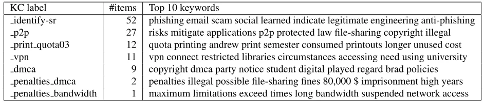
Table 2: Top 10 keywords extracted from the body only of a sample of knowledge components of various sizes.

We first illustrate this on thenoSAKC model, for which we can use the minimally descriptive KC la-bels as partial reference. Table 2 shows the top key-words extracted from the body text for a sample of knowledge components. Even for knowledge com-ponents with very few items, the extracted keywords are clearly related to the topic suggested by the label. Although the label itself is not available when es-timating the model, words from the label often ap-pear in the keywords (sometimes with slight mor-phological differences). Our first metric evaluates the quality of the extraction by the number of times words from the (unknown) label appear in the key-words. For the model in Table 2, this occurs in 44 KCs out of the 108 in the model (41%). These KCs are associated with 280 items (34%), suggesting that labels are more commonly found within keywords for small KCs. This may also be due to vague labels for large KCs (e.g.identify,srin Table 2), although the overall keyword description is quite clear ( phish-ing,email,scam).

We now focus on two ways to evaluate keyword quality:diversity(number of distinct keywords) and

specificity(how many KC a keyword describes). De-sirable keywords are specific to one or few KCs. A side effect is that there should be many different key-words. We therefore compute 1) how many distinct keywords there are overall, 2) how many keywords appear in a single KC, and 3) the maximum number of KCs sharing the same keyword. As a baseline, we compare against the simple strategy that consists in simply picking as keywords the tokens with max-imum probability in the KC profile (1). This base-line is common practice when describing probabilis-tic topic models (Blei et al., 2003).

Table 3 compares KL score (“KL-*” rows) and maximum probability baseline (“MP-*” rows) for

the two KC models. The total number of keywords is fairly stable as we extract up to 10 keywords per KC in all cases (some KCs have a single item and not enough text). The KL rows clearly show that our KL-based method generates many more differ-ent keywords than MP, implying that MP extracts the same keywords for many more KCs.

• With KL, we have up to 727 distinct keywords (out of 995) fornoSA and 372 out of 440 for

C75, i.e. an average 1.18 to 1.37 (median 1) KC per keyword. With MP the keywords de-scribe on average 3.1 KC ofnoSA, and 2.97 of

C75.

• With KL, as many as 577 (i.e. more than half) keywords appear in a singlenoSAKC. By con-trast, only as few as 221 MP keywords have a unique KC. For C75, the numbers are 316 (72%) vs, 88 to 131.

• With KL, no keyword is used to describe more than 9 to 19noSAKCs and 6 to 12C75KCs. With MP, some keywords appear in as many as 87noSAKCs and all 44C75KCs. This shows that they are much less specific at describing the content of a KC.

These results all point to the fact that the KL-based method provides better diversity as well as speci-ficityin naming the different KCs.

model total diff. uniq. max

KL-body 995 727 577 9

KL-b+h 1005 722 558 10

noSA KL-all 1080 639 480 19

MP-body 995 534 365 42

MP-b+h 1005 521 340 34

MP-all 1080 352 221 87

KL-body 440 372 316 6

C75 KL-all 440 328 254 12

MP-body 440 203 131 33

MP-all 440 148 88 44

KL-body 440 377 325 4

C75 KL-all 440 332 261 11

(+sw) MP-body 440 76 43 43

MP-all 440 68 32 44

Table 3: Statistics on various keyword extraction meth-ods. KL (Kullback-Leibler score) and MP (maximum probability) are tested on body only, body+hints (b+h) or all text. We report the total number of keywords ex-tracted (Total), the number of different keywords (diff.), keywords with unique KC (unique) and maximum num-ber of KC per keyword (max). “+sw” indicates stopwords are included (not filtered).

very similar across items. They add textual informa-tion but tend to smooth out profiles. This is shown in the comparison between “KL-body” and “MP-all” in Table 4. The latter extracts “correct” and “incor-rect” as keywords for most KCs in both models, be-cause these words frequently appear in the response feedback (Fig. 1). KL-based naming discards these words because they are almost equally frequent in all KCs and are not specific enough. Table 4 also shows that MP selects the same frequent words for both KC models. By contrast, the most used KL keywords fornoSAare not so frequently used to de-scribeC75KCs, suggeting that the descriptions are more specific to the models.

Impact of stopwords: The bottom panel of table 3 (indicated by “(+sw)”) shows the impact of not filtering stopword on the keyword extraction met-rics (i.e. keeping stopwords). For KL the impact is small: filtering out stopwords actually degrades per-formance slightly. The impact on MP is massive: there are up to three times less different keyword (76 vs. 203), and most are high-frequency function words (“to”, “of”, etc.). The extreme case is “the”,

KL-body MP-all

Keyword #no #C Keyword #no #C

use 9 1 incorrect 87 44

following 8 1 correct 67 41

access 7 - review 49 22

andrew 7 2 information 30 20

account 7 - module 29 9

search 7 2 course 26 9

Table 4: Keywords associated with most KCs innoSA, with number of associated KC innoSA(#no) andC75

(#C). Left: KL score on item body; Right: max. proba-bility on all text.

extracted forall44 KCs. Results onnoSAare simi-lar and not included for brievity.

6 Discussion

We described a simple probabilistic method for knowledge component naming using keywords. This simple method is effective at generating de-scriptive keywords that are both diverse and spe-cific. We show that our method clearly outperforms the simple baseline that focuses on most probable words, with no impact on computational cost.

Although we only extract keywordsfrom the tex-tual data, one straightforward improvement would be to identify and extract either multiword terms, which may be more explanatory, or relevant snip-pets from the data. A related perspective would be to combine our relevance scores with, for example, the output of a parser in order to extract more compli-cated linguistic structure such as subject-verb-object triples (Atapattu et al., 2014).

Acknowledgement

We used the ’OLI C@CM v2.5 - Fall 2013, Mini 1 (100 students)’ dataset accessed via DataShop (Koedinger et al., 2010). We thank Alida Skogsholm from CMU for her help in choosing this dataset.

References

T. Atapattu, K. Falkner, and N. Falkner. 2014. Acquisi-tion of triples of knowledge from lecture notes: A nat-ural language processing approach. In7th Intl. Conf. on Educational Data Mining, pages 193–196. T. Barnes. 2005. The Q-matrix method: Mining student

response data for knowledge. In AAAI Educational Data Mining workshop, page 39.

M. Birenbaum, A. E. Kelly, and K. K. Tatsuoka. 1992.

Diagnosing Knowledge States in Algebra Using the Rule Space Model. Educational Testing Service Princeton, NJ: ETS research report. Educational Test-ing Service.

David M. Blei, Andrew Y. Ng, and Michael I. Jordan. 2003. Latent dirichlet allocation. Journal of Machine Learning Research, 3(Jan):993–1022.

Y. Chen, J. Liu, G. Xu, and Z. Ying. 2014. Statisti-cal analysis of Q-matrix based diagnostic classification models. Journal of the American Statistical Associa-tion.

M. Desmarais, B. Beheshti, and P. Xu. 2014. The re-finement of a Q-matrix: Assessing methods to validate tasks to skills mapping. In7th Intl. Conf. on Educa-tional Data Mining, pages 308–311.

M. Desmarais. 2011. Mapping questions items to skills with non-negative matrix factorization. ACM-KDD-Explorations, 13(2):30–36.

E. Gaussier, C. Goutte, K. Popat, and F. Chen. 2002. A hierarchical model for clustering and categorising doc-uments. InAdvances in Information Retrieval, pages 229–247. Springer Berlin Heidelberg.

M.J. Gierl, J. P. Leighton, and S. M. Hunka. 2000. Ex-ploring the logic of Tatsuoka’s rule-space model for test development and analysis. Educational Measure-ment: Issues and Practice, 19(3):34–44.

K.R. Koedinger, R.S.J.d. Baker, K. Cunningham, A. Skogsholm, B. Leber, and J. Stamper. 2010. A data repository for the EDM community: The pslc datashop. In C. Romero, S. Ventura, M. Pechenizkiy, and R.S.J.d. Baker, editors,Handbook of Educational Data Mining. CRC Press.

A.S. Lan, A.E. waters, C. Studer, and R.G. Baraniuk. 2014. Sparse factor analysis for learning and con-tent analytics. Journal of Machine Learning Research, 15:1959–2008, June.

J. Liu, G. Xu, and Z. Ying. 2012. Data-driven learn-ing of Q-matrix.Applied Psychological Measurement, 36(7):548–564.

A. McCallum and K. Nigam. 1998. A comparison of event models for naive Bayes text classification. In

AAAI-98 workshop on learning for text categorization, pages 41–48.

J.C. Stamper and K.R. Koedinger. 2011. Human-machine student model discovery and improvement using DataShop. InArtificial Intelligence in Educa-tion, pages 353–360. Springer Berlin Heidelberg. Y. Sun, S. Ye, S. Inoue, and Yi Sun. 2014. Alternating

recursive method for Q-matrix learning. In 7th Intl. Conf. on Educational Data Mining, pages 14–20. K.K. Tatsuoka. 1983. Rule space: an approach for

deal-ing with misconceptions based on item response the-ory.Journal of Educational Measurement, 20(4):345– 354.