Choosing put option parameters based
on quantiles from the distribution of
portfolio value
Bell, Peter Newton
University of Victoria
9 September 2014
Choosing put option parameters based on quantiles from the distribution of portfolio value
Peter N. Bell
University of Victoria
The author gratefully acknowledges support from the
Social Science and Humanities Research Council through the
Joseph-Armand Bombardier Canada Graduate Scholarship-Doctoral award.
The author also acknowledges the IMT Institute for Advanced Studies Lucca
for accommodation and support while conducting the research described here.
Abstract
This paper explores how a put option changes the probability distribution of portfolio
value. The paper extends the model introduced in Bell (2014) by allowing both the
quantity and strike price to vary. I use the 5% quantile from the portfolio distribution to
measure riskiness and compare different put options. I report a so-called ‘quantile surface’ that shows the quantile across different combinations of quantity and strike price. I find
that it is possible to maximize the quantile by purchasing a put with quantity equal to one
and strike deep in the money; however, the distribution with such a put option collapses to
a single point because the option hedges all variation in stock price. This result is
analogous to full-insurance in insurance economics, but has practical limitations. The
quantile surface also shows that certain put options will decrease the quantile, which is
equivalent to increasing the riskiness of the portfolio, and leads me to ask: what return will
an investor receive in return for bearing that extra risk? I find that one such put option will
cause the distribution to have an asymmetric shape with positive skewness, which is
interesting to some speculators.
Keywords: Portfolio, put option, probability distribution, quantile, optimization,
Use of quantiles from the distribution of portfolio value to choose put option parameters
This paper is concerned with the use of financial derivatives. I use a simple, toy
model introduced in Bell (2014) where an agent holds one unit of put option and is allowed
to trade some quantity of (at the money) put options. Here, I extend the model to consider
choice of both quantity and strike price. Suppose that an agent holds some dollar value of
stock, for example one unit of stock worth $100. In my model, quantity refers to the
notional amount of the put option in proportional to dollar value of stock: if quantity equals
two (Q=2), then the agent holds put options with notional value of $200. The strike price
refers to the level at which the put option begins to offset losses in the stock price. There is
an analogy between the put option in my model and an insurance contract, but I focus on
the context of financial derivatives in this short paper.
The paper uses simulation to generate insight into the model since it has no clear
analytic solution. I use the same data generating process as in Bell (2014): the initial stock
price is 100 and the price at option-expiry is governed by a log-normal distribution with
mean zero and standard deviation 10%. This is a plain, vanilla model in financial
economics that allows me to use the Black-Scholes option pricing formula for all options in
the paper. I overlook concerns such as volatility smiles, where options deep out of the
money have larger prices, or potential illiquidity of some deep in the money options.
One of striking results from Bell (2014) is associated with so-called quantile
preferences. The 5% quantile from distribution of portfolio value is based on the Value at
Risk measure used in market risk assessment: it represents an extremely low level for the
portfolio, a value for which the portfolio will be larger with 95% confidence (in context of
the model). Bell (2014) reported that the optimal quantity of put options based on quantile
preferences is always precisely equal to one (Q=1.0), which was striking because it is a
knife-edge result that is robust to resampling. This result inspired me to investigate the
The quantile surface
The quantile surface refers to a mathematical object that shows how the portfolio
distribution changes with different types of put options. The put options are defined by
two choice variables: quantity and strike price. I use a discrete approach to estimate the
surface as follows. I specify a set of values for each choice variables and create a grid,
where each point represents a put option. I estimate the probability distribution for the
portfolio at each grid point and use the quantile from each distribution to determine the
height of the surface at that grid point. I specify a generous range for each choice variable
in order to explore the global behaviour of the quantile surface: I allow quantity to vary
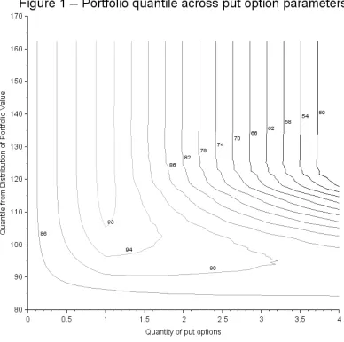
between 0 and 4, and strike price to vary between 80 and 160. I display the quantile
surface as a level set diagram (topographical map) in Figure 1.
Figure 1 shows some level sets for the quantile surface. Each line has a
corresponding numeric label, which specifies the value of the quantile for all combinations
of quantity and strike price along the line. Higher values for the quantile are associated
with less risk in the portfolio. The diagram shows several interesting features, which I
discuss before characterizing the types of put options that are associated with the maximal
value for the quantile.
One feature of interest in Figure 1 is the fact that the level sets become vertical lines
for large values of the strike price (above 130 on vertical axis). This occurs because a put
option with high strike will always expire in the money: the underlying normal probability
model means that prices are almost surely less than 130. If the put option always expires
in the money, then increasing the strike price further does not have any net effect within
the model because the increased payoff is offset by increased price. The parallel level sets
for high strikes suggest that changing strike price is inconsequential in this region.
The second feature of interest is the shape of the level set for lower strike prices.
The negative slope for level sets suggests there is some tradeoff between quantity and
strike, where an agent can achieve similar risk-management goals by increasing quantity
and decreasing strike price, or vice versa. However, the tradeoff is non-constant based on
In Bell (2014), I identify the quantity of put options that maximizes the quantile. It
is possible to do so again with quantile surface, even though it may not be clear from Figure
[image:6.612.99.487.109.495.2]1. To help clarify, I show the shape of the quantile surface around the optimum in Table 1.
Table 1 -- Shape of quantile surface around optimum
Strike price
Quantity
100 110 120 130 140 150
0.8 93.64 96.07 96.71 96.82 96.83 96.83
1 96.01 99.05 99.85 99.98 100.00 100.00
Table 1 shows that an agent can force the quantile to equal 100 if they buy an option
with quantity equal to 1.0 and strike above 140. Any strike above 140 will ensure this
result because the level sets are vertical lines, as discussed above. This implies that there is
not one single put option that maximizes the quantile, instead there is a continuous set of
‘optimal’ put options that have quantity equal to one and strike deep in the money. This occurs because such put options hedge all variation in the stock price: the delta is
approximately equal to negative one when they first buy the put option, and the option
always expires in the money because the strike is so deep in the money.
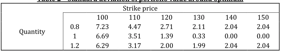
Although Table 1 reveals that the optimal put option causes the quantile to equal
100, it does not provide any further information about the shape of distribution when
using these options. Table 2 shows that the standard deviation of the optimal portfolio
value approaches zero: the distribution collapses to a single point. Again, this occurs
because such a put option hedges all variation in stock price – both upward and downward movement. It could be said that the optimal put option causes the portfolio to be ‘globally
[image:7.612.70.549.415.502.2]flat’, in contrast to the phrase ‘locally flat’ used by risk management professionals.
Table 2 – Standard deviation of portfolio value around optimum
Strike price
Quantity
100 110 120 130 140 150
0.8 7.23 4.47 2.71 2.11 2.04 2.04
1 6.69 3.51 1.39 0.33 0.00 0.00
1.2 6.29 3.17 2.00 1.99 2.04 2.04
The results in this section show that an agent can use a put options to control the
quantile from the distribution of portfolio value. Furthermore, if they want to maximize
this quantile then they will buy one unit of put options (proportional to stock position)
with strike deep in the money and this option will eliminate all variation in portfolio value
in context of the model. This is an extreme result, but it has some precedent in insurance
economics where a risk averse agent chooses full insurance under risk neutral pricing, as
Further inspection of the quantile surface in Figure 1 shows that there exists a
region where the level sets become very close together (quantity from 2.0 to 4.0 and strike
from 100 to 125). When the level sets are close together, the surface is very steep. This
region raises concerns because it allows an agent to decrease the quantile, or increase the
risk in their portfolio, which leads me to ask what sort of return they get in exchange for
the increase in risk? To explore this region, I consider one portfolio with quantity equal to
Figure 2 compares two different distributions of portfolio value. The dark line
represents the probability distribution when the agent buys a put option from the region
where the quantile surface is steep. I refer to this as a ‘Speculative distribution’ because it has a triangular, wedge shape. In contrast, the light gray line represents the distribution
when the agent buys no options: by construction, the distribution has a normal, bell shape.
There are several important differences between these two distributions.
Figure 2 shows that the speculative distribution has a larger, longer right tail than
the benchmark distribution. This means that the speculator is more likely to get larger
portfolio values. Figure 2 also shows that the speculative distribution has a smaller left tail,
which is truncated at 85. This means that the speculator will not ever have as severely low
values as the benchmark distribution. Together, this extended upside and reduced
downside suggest that the speculative distribution reflects a particular combination of
attributes that appeals to certain speculators: asymmetric returns with positive skewness.
Mark Spitznagel (2013) describes how this concept is valuable inside finance, from futures
trading in the pit to electronic trading in tail options, and outside of finance, as in ecology
and ancient Chinese military philosophy.
Table 3 -- Positive skewness for speculative portfolio
Pearson's moment skewness coefficient 0.98 Pearson's median skewness coefficient 0.72
Table 3 shows that the speculative distribution does, indeed, have positive
skewness. This result provides technical evidence to support the claim of asymmetric
returns with positive skewness above. However, these results do not imply that the
speculative distribution is necessarily superior to the benchmark. The quantiles for each
distribution are very similar, approximately 82 for the speculative distribution and 84 for
the benchmark distribution, but the shapes of the two distributions are very different.
Notice that the peak of the speculative distribution is more pronounced and actually to the
left of the benchmark distribution; this means the speculative portfolio will generally
provide lower returns than the benchmark. In terms of decision theory, neither
This short paper investigates a model where an agent holds one unit of stock and is
allowed to buy a put option on the stock with some quantity and strike price. The agent
uses the 5% quantile from the distribution of portfolio value to asses if the particular put
option reduces risk in the portfolio or not. I report the quantile surface, which shows how
the quantile varies across a grid of values for quantity and strike. The surface shows that
there exists a set of put options with quantity one and strike deep in the money, that
maximize the quantile and reduce all variation in the portfolio value. Such put options
could be said to reduce all the risk in the portfolio, but they may be very illiquid in practice.
I also investigate a region of the quantile surface where the surface has the steepest
gradient. I pick a put option from this region (quantity 3.0 and strike 105) that gives a
similar value for the quantile as the benchmark case and compare the two portfolio
distributions. I find that the distribution with the put option has properties that appeal to
some speculators, asymmetric returns with positive skewness, which suggests that
maximizing the quantile is not an appropriate objective for all types of agents.
In conclusion, I will identify two areas for further work. One is to replace the
quantile measure used here with other types of utility functions or risk measures. The
underlying distribution for portfolio values will be the same, but different measures may
lead to different insights; for example, what is the tradeoff between strike price and
quantity of put option for an agent with a risk averse utility function? The second direction
of further work is to better develop the concept of time. The model used here only has two
time periods, when the agent first buys the option and when the option expires. However,
contemporary options markets have monthly term structures, which implies that there are
is another entire dimension for the put options: expiry time. It will be a challenge to
incorporate multiple expiry times into the model as described here, but it could provide
References
Bell, P.N. (2014). Optimal use of put options in a stock portfolio. Unpublished manuscript.
Available from http://mpra.ub.uni-muenchen.de/54871/
Spitznagel, M. (2013). The Dao of Capital: Austrian Investing in a Distorted World.
// Code Appendix for 'Choice of Put Option Parameters' paper. // By Peter Bell, September 2014, written in SciLab 5.5.
// Section 1: Calculate level set for 5% quantile across strike, quantity // Also creates Figure 1
clear
nSamp=1000; sigma=0.1; initPrice=100; rate=0; diffRet=rand(nSamp,1,"normal");
priceExp=initPrice*exp(diffRet*sigma);
for quantCount =1:100
for strikeCount =1:175
quantLoop=quantCount/25; strikeLoop=75+strikeCount/2;
d1=(1/sigma)*( log(initPrice/strikeLoop) + (rate+sigma^2/2) ); d2=d1 - sigma;
[p1,q1]=cdfnor("PQ",-d1,0,1); [p2,q2]=cdfnor("PQ",-d2,0,1);
putPrice=strikeLoop*exp(-rate)*p2-initPrice*p1; // Using Black-Scholes price
for i=1:nSamp
portUnit(i)=priceExp(i)+quantLoop*(-putPrice+... max(strikeLoop-priceExp(i),0));
end
// Construct payoff as-if bought particular put option quantileVecTemp=gsort(portUnit);
quantileMatrixResult(quantCount,strikeCount)=... quantileVecTemp(nSamp*0.95);
// Key object is 'quantileMatrixResult' because // shows 5% quantile portfolio with each put option end
end
quantVec=(1:100)/25; strikeVec=75+(1:175)/2; quantLevel=50:4:110; f=get("current_figure");
f.figure_size=[800,800] // Size of full window f.color_map =graycolormap(16); scf(0);
contour2d(quantVec,strikeVec,quantileMatrixResult,quantLevel);
xtitle("Figure 1 -- Portfolio quantile across put option parameters", ... 'Quantity of put options',...
axesCurr.font_size=3; title_label=axesCurr.title; title_label.font_size=5; x_label=axesCurr.x_label; x_label.font_size=3; y_label=axesCurr.y_label; y_label.font_size=3;
xs2bmp(0,'Fig1.bmp'); // Creates Figure 1 from paper
// Section 2: Show behaviour of quantile around optimum parameter values // Look at Q from 0.8 to 1.2 and K from 100 to 150.
for quantCount =1:3
for strikeCount =1:6
quantLoop=0.6+0.2*quantCount; strikeLoop=90+10*strikeCount;
d1=(1/sigma)*( log(initPrice/strikeLoop) + (rate+sigma^2/2) ); d2=d1 - sigma;
[p1,q1]=cdfnor("PQ",-d1,0,1); [p2,q2]=cdfnor("PQ",-d2,0,1);
putPrice=strikeLoop*exp(-rate)*p2-initPrice*p1; for i=1:nSamp
portUnit(i)=priceExp(i)+quantLoop*(-putPrice+... max(strikeLoop-priceExp(i),0));
end
quantileVecTemp=gsort(portUnit);
quantileTable(quantCount+1,1)=quantLoop; quantileTable(1,strikeCount+1)=strikeLoop; quantileTable(quantCount+1,strikeCount+1)=... quantileVecTemp(nSamp*0.95);
// This is quantile around optimum devTable(quantCount+1,1)=quantLoop; devTable(1,strikeCount+1)=strikeLoop; devTable(quantCount+1,strikeCount+1)=... stdev(portUnit);
// This is standard deviation of wealth around optimum end
end
csvWrite(quantileTable, 'Table1.csv');
csvWrite(devTable, 'Table2.csv');
// Tables 1 and 2 help characterize the character of the optimum
// Section 3: Show distribution for one interesting portfolio
strike=105; quantPut=3;
nSamp=10000; sigma=0.1; initPrice=100; rate=0; diffRet=rand(nSamp,1,"normal");
priceExp=initPrice*exp(diffRet*sigma);
d1=(1/sigma)*( log(initPrice/strike) + (rate+sigma^2/2) ); d2=d1 - sigma;
[p1,q1]=cdfnor("PQ",-d1,0,1); [p2,q2]=cdfnor("PQ",-d2,0,1);
putPrice=strike*exp(-rate)*p2-initPrice*p1;
for i=1:nSamp
portUnit(i)=priceExp(i)+quantPut*(... max(strike-priceExp(i),0)-putPrice);
end
skewVec = ( (portUnit-mean(portUnit))/stdev(portUnit) )^3; skewStat =mean(skewVec);
skewPearson =3*(mean(portUnit)-median(portUnit))/stdev(portUnit);
csvWrite([skewStat ; skewPearson] , 'Table3.csv'); // Table 3 shows the distribution has positive skewness
histplot(20,priceExp,style=[color("gray")])
histplot(20,portUnit)
hl=legend(['Benchmark distribution (no put option)'; ...
'Speculative distribution (Q=3,K=105)']);
xtitle("Figure 2 -- Comparison of speculative and benchmark distributions", ... 'Portfolio value at option expiry',...
'Probability of portfolio value'); axesCurr=get("current_axes"); axesCurr.font_size=3;
title_label=axesCurr.title; title_label.font_size=5; x_label=axesCurr.x_label; x_label.font_size=3; y_label=axesCurr.y_label; y_label.font_size=3; l=axesCurr.children(1); l.font_size =3;
xs2bmp(0,'Fig2.bmp'); // Creates Figure 2 from paper
// End of file.