Returning Home Analysis in Tokyo Metropolitan Area at the time of the Great East Japan Earthquake using Twitter Data

Returning-Home Analysis in Tokyo Metropolitan Area

at the time of the Great East Japan Earthquake using Twitter Data

Yusuke Hara

New Industry Creation Hatchery Center, Tohoku University 6-3-09 Aoba Aramaki Aoba-ku Sendai, Miyagi 980-8579, Japan

hara@plan.civil.tohoku.ac.jp

Abstract

This paper clarifies the occurrence fac-tors of commuters unable to return home and the returning-home decision-making at the time of the Great East Japan Earth-quake by using Twitter data. First, to ex-tract the behavior data from the tweet data, we identify each user’s returning-home behavior using support vector machines. Second, we create non-verbal explanatory factors using geotag data and verbal ex-planatory factors using tweet data. Then, we model users’ returning-home decision-making by using a discrete choice model and clarify the factors quantitatively. Fi-nally, by sensitivity analysis, we show the effects of the existence of emergency evac-uation facilities and line of communica-tion.

1 Introduction

The 2011 earthquake off the Pacific coast of To-hoku, often referred to in Japan as the Great East Japan Earthquake, was a magnitude 9.0 under sea megathrust earthquake that occurred at 14:46JST (05:46 UTC) on March 11, 2011. The focal re-gion of this earthquake was widespread, spanning approximately 500 km north to south from off the Ibaraki shore to the Iwate shore and approximately 200km east to west. The number of deaths and missing persons attributed to this disaster totaled more than 19,000, and the complex, large-scale disasters of the earthquake, tsunami, and nuclear power plant accident had a major impact on peo-ple’s lives. The Tokyo metropolitan area also was hit by a strong earthquake and various traffic prob-lems occurred. For example, many railway and subway services were suspended for maintenance. Therefore, almost every railway and subway user was unable to return home easily, and they were

called “victims unable to return home.” According to (Measures Council for Victims Unable to Re-turn Home by Earthquake that directly hits Tokyo Area, 2012), the number of people who were not able to go home during that day by paralysis of these transport networks is estimated about 5.15

million people and it is30%of a going-out people

of the day.

Assessing the problem of “victims unable to return home” in Tokyo metropolitan area is ex-tremely important for anti-disaster measures. Al-though the questionnaire is performed ex post, it is not yet shown clearly what made going-home decision-making after the earthquake disas-ter. Moreover, since it was going-home behavior in big confusion, the problem that detailed time and position information are unknown exist.

Some previously studies have examined human behaviors via analysis of behavior log data at the time of a large-scale disaster. Because no rapid and accurate method existed to track population movements after the 2010 earthquake in Haiti, (Bengtsson et al., 2011) used position data from subscriber identity module (SIM) cards from the largest mobile phone company in Haiti to estimate the magnitude and trends of population move-ments after the 2010 Haiti earthquake and the subsequent cholera outbreak. Their results indi-cated that estimates of population movements dur-ing disasters and outbreaks can be acquired rapidly and with potentially high validity in areas of high mobile phone usage. (Lu et al., 2012) also used the same data in Haiti to determine that 19 days after the earthquake, population movements had caused the population of the capital Port-au-Prince to de-crease by approximately 23% and that the destina-tions of people who left the capital during the first three weeks after the earthquake were highly cor-related with their mobility patterns during normal times and specifically with the locations of people with whom they had significant social bonds. Lu

et al. concluded that population movements dur-ing disasters may be significantly more predictable than previously thought. Overall, these previous studies clarified human movement over long pe-riods of time. They showed that people in areas affected by an earthquake take refuge temporarily and that the population in the affected area is re-covered over several months. Behavior log data should be able to clarify not only such long-term human behavior but also the human behaviors at the time of a disaster.

In this research, we analyze tweet data of Twit-ter as the behavior log data at the time of the Great East Japan Earthquake. Although tweet data does not contain actual behavior necessarily, there is possibility of containing thinking process and be-havioral factors. We clarify the factors of going-home behavior in case of the Great East Japan Earthquake using Twitter data.

2 From Tweet Data To Behavioral Data

2.1 Framework

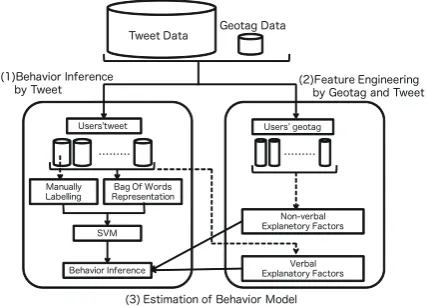
First, we provide a framework of this research to analyze users’ going-home behavior using tweet data and geotag data. Figure 1 shows our frame-work: (1) behavior inference by tweet data,(2) fea-ture engineering by geotag and tweet data, (3) es-timation of behavioral model.

In (1) behavior inference by tweet data part, we inferred users’ going-home behavior result us-ing Support vector machine (SVM) and Bag-Of-Words (BOW) representation. In (2) feature engi-neering by geotag and tweet data part, we made explanatory factors of users’ behavior from tweet

data and geotag data. In (3) estimation of

be-havioral model part, we estimated users’ behavior model (discrete choice model).

2.2 Data

In this section, we provide an outline of our data. This data is about 180-million tweet by Japanese in Twitter from March 11, 2011 to March 18, 2011. There are about 280 thousands tweet with geotag in this data. We sampled tweets whose timestamp is from 14:00, March 11 to 10:00, March 12 and whose GPS location is within Tokyo metropolitan area. The number of these tweet is 24,737 and the number of unique users (account) is 5,281. To observe users’ trip on the day, we ex-tracted users that had over 2 geotag tweet and the number of users is 3,307. We assume that these

Tweet Data Geotag Data

……… ………

Manually Labelling

(1)Behavior Inference

by Tweet (2)Feature Engineeringby Geotag and Tweet

Users tweet Users geotag

Bag Of Words Representation

SVM

Behavior Inference Explanatory FactorsVerbal Non-verbal Explanetory Factors

(3) Estimation of Behavior Model

Figure 1: Framework in this research

users can tweet about the Great East Japan Earth-quake and their going-home behavior. Therefore, we analyzed all tweet of these users from 14:00, March 11 to 10:00 (3,307 users, 132, 989 tweets). We tagged 300 users’ going-home behavior re-sult manually to make supervised data. Our label set is composed of 1) going home by foot, 2) by train, 3) staying their offices or hotels until tomor-row morning, 4) other choice (taxi, bus, etc.), 5) unclear.

2.3 Morphological analysis

Next, we give morphological analysis by MeCab and obtained BOW representation by each user’s tweet. To find the relationship between going-home behavior and each user’s tweet, we use in-formation gain. Inin-formation gain is index which shows decreasing degree of each class’s entropy

by existing wordw. If wordwis contained each

user’s tweet, Random variableXw equals 1 and

otherwiseXw = 0. Random variables which

in-dicates each class iscand entropyH(c)is written

as

H(C) =−∑

c

P(c) logP(c). (1)

And conditional entropy is written as

H(c|Xw = 1) =− ∑

c

P(c|Xw= 1) logP(c|Xw = 1)

H(c|Xw= 0) =− ∑

c

P(c|Xw= 0) logP(c|Xw= 0).

Information gainIG(w) of word wis defined as

average decreasing entropy and written as

Table 1: Illustrative examples of words whose in-formation gain is high

駅(station)歩い(walk)足(foot)休憩(rest)

自転車(bicycle)電車(train)ヤバイ(danger)

止まっ(stop)半分(half)到着(arrived)

1)by foot 歩ける(can walk)テレビ(TV)トイレ(toilet)

環七(Kan-nana Street) km川崎(Kawasaki)

疲れ(tired)遠い(far)道(road)

大江戸(O-edo subway line)入場(entry)

2)by train 田園都市線(Denen-toshi line)奇跡(miracle)

なんとか(luckily)順調(smoothly)

京王(Keio line)乗れ(can take a train)

泊め(sleep)朝(morning)総武線(Sobu line)

混雑(congested)検索(search) JR (JR line)

乗車(take a train)満員(full capacity)

3)stay 明け(daylight)暇(a spare time)

始発(first train in the morning)悩む(worry)

4)other Twitpic

5)unclear jishin，skype

We calculated all words information gain

IG(w) by 5 class (walk, train, stay, other,

un-clear). Table 1 shows illustrative examples.

For example, words whose conditional probabil-ity of walking is high are “half”, “far”, “km”, “Kawasaki” and “Kannana Street”. They show user’s location. And “toilet”, “tired” and “dan-ger” indicates psychological factors during going-home by foot.

In the case of train, “miracle”, “luckily” is con-tained and “O-edo line” and “Denen-toshi line” are the train and subway lines which is operated in March 11. In the case of stay, “morning”, “day-light” and “sleep” indicates that users slept at ho-tel or their offices and “first train in the morn-ing”, “worry” and “search” shows their going-home timing. Other choices users, who choose bi-cycle, taxi etc, and unclear users don’t show the understandable tendency. However, they submit-ted pictures for Twitpic, which is photo share site, and tweeted with #jishin hashtag.

As seen above, the words whose information gain is high is useful to infer their going-home behavior. Therefore, we made classifier by using these words as features.

2.4 SVM and behavior inference

In this section, we infer each user’s behavioral re-sult by SVM. we use 300 labeled data as super-vised data and we treat top 500 words of informa-tion gain as features of SVM. In learning, we did 9-fold cross validation and average accuracy rate is73.3%.

Figure 2 shows the inferred result. The number

0% 10% 20% 30% 40% 50% 60% 70% 80% 90% 100% Survey by Yuhashi

Survey by SRC Inference

by this research Walk (71.5%) Stay (15.1%)

People who could go home (80.1%)

People who could go home (78.6%)

Stay (19.9%)

Stay (9.9%) could not

(11.5%) Train (13.4%)

(n = 1052) (n = 2026) (n = 2672)

Figure 2: Inferred result and comparison of other survey

of users by foot is1,913, the number of users by

train is 359, the number of users staying is 385,

the number of users by other choice is15and the

number of users whose choice is unclear is 635.

This result indicates that the ratio of all

going-home users except unclear users is84,9%.

To discuss the accuracy of this inference sult, we compare our result with other survey re-sults. Figure 2 shows the survey result by (Sur-vey Research Center, 2011) and the sur(Sur-vey result

by (Yuhashi, 2012). The result of Survey

Re-search Center says 80.1% of all could get home

and the result of Yuhashi says78.6%of all could

get home.

3 Behavioral Analysis

3.1 Non-verval factors

Based on the prediction of going-home decision-making classified by user, nonverbal / verbal ex-planation factor is created from tweet data or geo-tag data, and the factor of each individual’s going-home decision-making is analyzed.

First, the explanation factor about travel behav-ior is created using the geotag data classified by user. In this research, for simplicity, we assume that a position before the earthquake is the lo-cation of office (origin) and a position of 12:00, March 12, 2011 is the location of home (destina-tion). Next, road network distance, the on foot time required, the station nearest office, the station nearest home, the railroad time required, railroad expense, and the number of times of a railroad change are created using these GPS data. These are the features created using the network at the time of usual.

Ikebukuro

Shibuya

Shinjuku Iidabashi

Tokyo

Nakameguro Meguro

Gotanda Shinagawa

Mita Roppongi

Suehirocho

Yokohama

Haneda Airport

Figure 3: Users’ location distribution before the earthquake

the direction of the suburban area.

Next, the cross tabulation result of going-home decision-making by the road network distance be-tween offices and houses is shown in Figure 5. This result indicates that the rate of on foot de-creases relatively as distance with a house be-comes long, but 50% or more of people got home on foot if their distance is 20 km over.

3.2 Verbal factors

Finally, a verbal explanation factor is gener-ated. Since it is surmised that a family’s exis-tence and with or without information has affected going-home decision-making, the factor which af-fects going-home decision-making behavior is ex-tracted from each user’s tweet.

First, we analyze the effect of a safety check with a family. In this research, the family was defined as a spouse and children living together. And 353 of 3,307 persons had spoken existence of a family living together. We extracted safety check tweet such as “I got e-mail from my wife! I felt easy,”, “The telephone led to the wife and the daughter at last! ” and “My telephone is not connected to my son’s nursery school. ”

Figure 6, 7 shows the time zone rate of the safety checked tweet and the safety unidentified tweet according to going-home decision making.

Safety checked tweets are concentrated before

Ikebukuro

Shinjuku Kichijoji

Shibuya

Tokyo

Gotanda Shinagawa Roppongi

Futakotamagawa

Shinmaruko

Yokohama

ShinyokohamaKawasaki Ueno

Kinshicho

Haneda Airport

Figure 4: Users’ location distribution in the morn-ing on March 12

1098 382 333 100

135 81 101 42

13 2 2 0

208 76 64 37

0% 20% 40% 60% 80% 100%

under 5km 5∼10km 10∼20km over 20km

by foot by train by other stay

Figure 5: The relationship between going-home behavior and the distance

18:00 (42% of on foot, 45% of by train, and 65% of stay). Safety unidentified tweets are also con-centrated before 18:00. We assume that the safety unidentified tweets are strongly reflecting each in-dividual’s psychological state because they can perform every time zone until safety checked. If we assume that the tweet in a earlier time zone is more important for each user, an on foot going-home person will regard his/her family’s safety unidentified situation as more questionable than a railroad going-home person, and he may make de-cision of going-home by foot.

rail-Tweet distribution 0 0.05 0.1 0.15 0.2 0.25 0.3 0.35 1 2 :0 0 1 3 :0 0 1 4 :0 0 1 5 :0 0 1 6 :0 0 1 7 :0 0 1 8 :0 0 1 9 :0 0 2 0 :0 0 2 1 :0 0 2 2 :0 0 2 3 :0 0 0 :0 0 1 :0 0 2 :0 0 3 :0 0 4 :0 0 5 :0 0 6 :0 0 7 :0 0 8 :0 0 9 :0 0 1 0 :0 0 1 1 :0 0 by foot by train stay time

Figure 6: The distribution of safety checked tweets

0 0.1 0.2 0.3 0.4 0.5 0.6 1 2 :0 0 1 3 :0 0 1 4 :0 0 1 5 :0 0 1 6 :0 0 1 7 :0 0 1 8 :0 0 1 9 :0 0 2 0 :0 0 2 1 :0 0 2 2 :0 0 2 3 :0 0 0 :0 0 1 :0 0 2 :0 0 3 :0 0 4 :0 0 5 :0 0 6 :0 0 7 :0 0 8 :0 0 9 :0 0 1 0 :0 0 1 1 :0 0 by foot by train stay Tweet distribution time

Figure 7: The distribution of safety unidentified tweets

road resumption tweet and going-home decision-making and it indicates that a railroad chooser tend to speak of railroad resumption information.

Finally, we analyze the relationship between individual psychological factor and going-home decision-making. On March 11, many utterances

about their mental situation were seen. Figure

9 shows the utterance rate of uneasy and going-home decision-making result. Interestingly, indi-viduals whose utterance rate of uneasy is under

5%tend to stay at office or hotel but people whose

utterance rate of uneasy is over 5% tend to go

home by foot. This results shows the person who felt fear tend to walk to home.

4 Behavioral Model

4.1 Discrete choice model

We built discrete choice model based on the ex-planatory variable generated in 3. Discrete choice model is a statistical model used in fields, such as econometrics, travel behavior analysis, and mar-keting, and is also called Random utility model ((Ben-Akiva and Lerman, 1985); (Train, 2003)). In this research, Multinomial Logit Model (MNL) is used and it is the most fundamental model in a discrete choice model.

Discrete choice models describe decision

mak-1696 158 59 211 101 47 10 4 1 282 86 17

0% 20% 40% 60% 80% 100%

ratio 0

ratio 0-0.1 ratio over 0.1

㼒㼛㼛㼠 㼠㼞㼍㼕㼚 㼛㼠㼔㼑㼞 㼟㼠㼍㼥

Figure 8: The relationship between the rate of rail-road resumption tweet and going-home decision-making 1563 180 170 273 72 14 9 6 260 95 30

0% 20% 40% 60% 80% 100%

ratio 0 ratio 0-0.05 ratio over 0.05

㼒㼛㼛㼠 㼠㼞㼍㼕㼚 㼛㼠㼔㼑㼞 㼟㼠㼍㼥

Figure 9: The relationship between uneasy tweet and going-home decision-making

ers’ choices among alternatives. A decision

maker, labeledn, faces a choice amongJ

alterna-tives. The decision maker would obtain a certain level of utility from each alternative. The utility

that decision makernobtains from alternativejis

Unj, j = 1, . . . , J. This utility is known to the decision maker but not, as we see in the following, by the researcher. The decision maker chooses the alternative that provides the greatest utility. The

behavioral model is therefore: choose alternativei

if and only ifUni > Unj, ∀j̸=i.

Consider now the researcher. The researcher does not observe the decision maker’s utility. The researcher observes some attributes of the alter-natives as faced by the decision maker, labeled

xnj ∀j, and some attributes of the decision maker,

labeledsn, and can specify a function that relates

these observed factors to the decision maker’s

util-ity. The function is denotedVnj =V(xnj, sn)∀j

and is often called representative utility. Usually,

V depends on parameters that are unknown to the

researcher and therefore estimated statistically.

Since there are aspects of utility that the

re-searcher does not or cannot observe, Vnj = Unj.

Utility is decomposed asUnj =Vnj+εnj , where

εnj captures the factors that affect utility but are

not included in Vnj. This decomposition is fully

general.

The researcher does not knowεnj∀jand

there-fore treats these terms as random. The joint

den-sity of the random vectorεn = (εn1, . . . , εnJ) is

denotedf(εnj). With this density, the researcher

makernchooses alternativeiis

Pni = Pr(Uni> Unj ∀j̸=i)

= Pr(Vni+εni > Vnj+εnj ∀j̸=i)

= Pr(Vni−Vnj > εnj−εni∀j̸=i)(3)

This probability is a cumulative distribution, namely, the probability that each random term

εnj−εniis below the observed quantityVni−Vnj.

MNL model is derived under the assumption that the unobserved portion of utility is distributed iid extreme value.

f(εnj) = e−εnje−e

−εnj

(4)

F(εnj) = e−e

−εnj

(5)

And decision makernchooses alternativeiis

de-rived as

Pni= eVni ∑

jeVnj

. (6)

This is choice probability of MNL model.

4.2 The setting of utility function

In discrete choice model, observed utility termVni

is generally defined asVni = β′xni. βis

coeffi-cient vector andxniis explanatory vector of

deci-sion makern’s alternativei.

In this research, data set is 2672 samples identi-fied by SVM except persons unclear and choice set is on foot, train, other and stay. Explanatory vari-ables of on foot are required time by foot, the ratio of uneasy tweets and alternative specific constant. Explanatory variables of train are required time by train, log of the distance between office and home, the ratio of train resumption tweets, the dummy variables of family safety checked tweets and al-ternative specific constant. Explanatory variables of stay are the ratio of uneasy tweets, the ratio of waiting position tweets, the dummy variables of family safety checked tweets and alternative spe-cific constant. We normalized the utility of other to 0.

Next, we outlines the estimation method of the coefficient parameter of a utility function. MNL model’s likelihood function is written as

LL(β) =

N

∑

n=1

∑

i

δnilnPni (7)

whereδniis Kronecker delta if decision maker n

choice i, δni = 1 and otherwise δni = 0. This

Table 2: The estimation result of MNL model

variables estimator t-value

required time (min/10) [foot, train] -0.012 -2.20

log(distance(km)) [train] 0.36 5.50

the ratio of train resumption [train] 4.17 5.72

the ratio of train uneasy [foot] 6.05 2.71

the ratio of train uneasy [stay] 4.52 1.82

the ratio of waiting position [stay] 2.98 4.52

family safety checked [train, stay] 1.14 3.54

alternative specific constant [foot] 4.88 18.50

alternative specific constant [train] 2.46 8.48

alternative specific constant [stay] 3.08 11.61

observations 2672

initial log likelihood -3704.179

final log likelihood -2107.771

likelihood ratio index(ρ2_{) 0.428}

likelihood function is globally concave (McFad-den, 1974). Therefore, parameters can be mated uniquely with a maximum likelihood esti-mation.

4.3 the results and simulation

Under the above setting, the estimation result is

shown in Table 2. A likelihood ratio index is0.428

and its goodness of fit is good enough. Moreover, the result that the coefficient parameter of the re-quired time is negative and the choice probability of train increases as the distance between office and home is far is suitable for basic analysis and intuition,

Moreover, we estimated parameters of the rate of the uneasy tweet separately by on foot and stay. It turns out that the uneasy tweet rate has had big-ger influence to on foot choice. For example, from

the ratio of parameters, the increase of5point

un-easy tweet ratio is equivalent to the increase of64

minutes required time by foot. From a perspective of family safety check, decision maker who could check family’s safety tend to choice stay. There-fore, family’s safety check is the important factors for the avoidance of confusion at the great disaster. A sensitivity analysis is conducted based on this result. One is the analysis of the effect of the exis-tence of a stay place on going-home behavior and another is the analysis of effect of family’s safety check in the early time zone. Figure 10 shows the results.

69.0 69.4 71.6

14.7 13.0 13.4

15.8 17.0 14.4

0% 20% 40% 60% 80% 100%

㼒㼛㼛㼠 㼠㼞㼍㼕㼚 㼛㼠㼔㼑㼞 㼟㼠㼍㼥

Current State

The effect of waiting location

The effect of safety check

Figure 10: The result of sensitivity analysis

times and the share of stay is17.0%.

On the other hand, the share of going-home

be-havior such as on foot and train decreases by3%.

Although3%of reduction seems to be very small

influence apparently, generally the traffic conges-tion and confusion in a transport system occur by

exceeding only 10 %of supplied capacity. From

this point,3%of reduction effects is not few.

Next, we analyzed the influence of the safety

check within a family. It is checked from the

tweets that there are 353 decision makers who have family living together. When all of these 353 persons was able to check family’s safety by 17:00, as shown in Figure 10, the number of agents who choice train or stay increase by 1.1 times, and the number of people who go home by foot de-crease by 0.95 time. Needless to say, the safety check within a family at the time of a disaster is the important information. Since lines of commu-nication other than a mobile phone carried out the big contribution by this earthquake disaster, these communication tools can prevent the confusion of transport network partially.

5 Conclusions

In this paper, we inferred the going-home behav-ior in Tokyo metropolitan area after the Great East Japan Earthquake using tweet data and geotag data of Twitter and clarified the decision-making fac-tors. Although the inference method of going-home behavior and the behavioral model were the existing techniques, by combining two data sources and techniques, the going-home behavior for each individual and its factors were clarified only from Twitter data. And the virtual scenario simulation was carried out and we analyzed the ef-fect of waiting space and communication tools.

In the ex post survey about the behavior in the earthquake disaster, the orders of samples is about thousands of people. In this research, the number of users whose tweets were with geotag is 3,307 people in Tokyo metropolitan area and it is also same order. However, if we can calculate the

sim-ilarity of users who have geotag and not have geo-tag from the similarity of users’ tweet, human be-haviors in the great disaster can be clarified in hun-dreds thousands of people’s order. We would like to consider these approach as future tasks.

Acknowledgments

We specially thank the Great East Japan Earth-quake Big Data Workshop and Twitter Japan.

References

Ben-Akiva, M. and Lerman, S. 1985. Discrete Choice Analysis: Theory and Application to Travel De-mand. MIT Press, Cambridge, MA.

Bengtsson, L., Lu, X., Thorson, A., Garfield, R., von Schreeb, J. 2011. Improved Response to Disasters and Outbreaks by Tracking Population Movements with Mobile Phone Network Data: A Post-Earthquake Geospatial Study in Haiti. PLoS Medicine, 8(8), e1001083.

Lu, X., Bengtsson, L. and Holme, P. 2012. Predictabil-ity of population displacement after the 2010 Haiti earthquake. Proceedings of the National Academy of Sciences of the United States of America, 109(29), 11576–11581.

McFadden, D. 1974. Conditional logit analysis of qualitative choice behavior. Frontiers in Economet-rics, Academic Press, New York, 105–142.

MeCab Yet Another Part-of-Speech and Morphological Analyzer, http://mecab.sourceforge.net/.

Train, K. 2003. Discrete Choice Methods with Simu-lation. Cambridge University Press, Cambridge.

Survey Research Center. 2011. Survey of the Great East Japan Earthquake disaster (“victims unable toreturn home”).

http://www.surece.co.jp/src/press/backnumber/ 20110407.html.

Measures Council for Victims Unable to Return Home by Earthquake that directly hits Tokyo Area. 2012. Measures Council for Vic-tims Unable to Return Home by Earthquake that directly hits Tokyo Area Final Report. http://www.bousai.metro.tokyo.jp/japanese/tmg/ kitakukyougi.htm.