Remarks on Testing Probabilistic Processes

Remarks on Testing Probabilistic Processes

Yuxin Deng

_{Rob van Glabbeek}

_{Matthew Hennessy}

Carroll Morgan

_{Chenyi Zhang}

A_{National ICT Australia, Locked Bag 6016, Sydney, NSW 1466, Australia}

B_{School of Computer Science and Engineering, The University of New South Wales, Sydney, Australia}

C_{Department of Informatics, University of Sussex, Falmer, Brighton, BN1 9QN, UK}

Abstract

We develop a general testing scenario for probabilistic processes, giving rise to two theories: probabilistic may testingandprobabilistic must testing. These are applied to a simple probabilistic version of the process calculus CSP. We examine the algebraic theory of probabilistic testing, and show that many of the axioms of standard testing are no longer valid in our probabilistic setting; even for non-probabilistic CSP processes, the distinguishing power of probabilistic tests is much greater than that of standard tests. We develop a method for deriving inequations valid in probabilistic may testing based on a probabilistic extension of the notion ofsimulation. Using this, we obtain a complete axiomatisation for non-probabilistic processes subject to probabilistic may testing.

Keywords: Probabilistic processes, nondeterminism, CSP, transition systems, testing equivalences, simulation, complete axiomatisations, structural operational semantics

1

Introduction

Operational semantics has played a useful role in computer science since the very inception of the subject [Lan63,ER64,Luc71,BJ78]. But with the publication of [Plo81] (republished as [Plo04]) came the realisation that, properly structured, op-erational semantics provides an elegant compositional method for specifying the semantics of programming languages. Because of its mathematical foundations, structural operational semantics can also be used to reason about the behavioural properties of programs, to the extent it even brings into question the necessity of denotational semantics.

Nowhere is the power of operational semantics more evident than in the develop-ment of process calculi: the semantic theory underlying CCS [Mil89], bisimulation 1 _{We acknowledge the support of the Australian Research Council (ARC) Grant DP034557.}

equivalence, is founded entirely on operational semantics. It provides powerful co-inductive proof methods for establishing process equivalences; it also supports compositional and algebraic reasoning techniques.

With CSP [Hoa85] the story is somewhat different: the failures model [BHR84] is denotational and was used to justify the algebraic laws so characteristic of the subsequent development of CSP as a specification language for processes. However, it later became apparent that, just as for CCS, this model and its algebraic theory could be fully justified using purely operational concepts based on notions of process testing [OH86,DH84]. So with CSP we have the best of all possible worlds:

• _{a denotational model,} • _{an operational model and} • _{an algebraic theory,}

all of which are in some sense equivalent.

The topic of this paper is probabilistic process calculi. The various semantic approaches for standard process calculi are essentially theories of nondeterministic

processes, where the nondeterminism represents possible choices that can be re-solved in a wholly unpredictable way. With probabilistic constructs the resolution becomes predictable up to a point, in that it is quantified; but the interaction be-tween the quantified and unquantified forms of choice then requires close attention. The issue is mainly that the two forms of choice differ, not that one is quantified and the other is not: for example, a similar effect occurs when considering demonic and angelic choice together. Because they differ it is necessary to consider carefully the order in which they occur, and how they might or might not distribute over each other.

The first papers on probabilistic process calculi [GJS90,Chr90,LS92] proceed by replacing nondeterministic with probabilistic choice. The reconciliation of non-deterministic and probabilistic choice starts with [HJ90] and has received a lot of attention in the literature [JL91,WL92,JHW94,SL94,Low93,Low95,Seg95,MMSS96, PLS00,BS01,JW02,SV03], even in the sequential world [HSM97,MMS96], and, more recently, within general semantic domains [MM01,Mis00,MOW04,TKP05,VW06]; as such it could be argued that it is one of the central problems of the area. And CSP makes the issue more interesting still, by having two forms of choice already (both internal and external), so that probabilistic choice becomes the third. The emphasis in this paper is on the development of an algebraic theory. Following [WL92] we adapt the original idea of testing [DH84] to probabilistic processes, ar-riving at two refinement relations between processes, theprobabilistic may preorder

and theprobabilistic must preorder. For example P ⊑pmay Qmeans that the prob-ability thatQmight pass a test is at least as good as the probability thatP might pass it. We then apply this general framework of probabilistic testing to a simple finite probabilistic process algebra,pCSP, obtained by adding a probabilistic choice operator to a cut-down version of CSP. In order to do so we first need to interpret

interactions which processes may have with their users.

With these generalisations it turns out that very few of the attractive algebraic laws underlying the algebraic theory of CSP, and indeed its denotational model, remain valid in the presence of probabilistic choice; this is demonstrated by a series of counterexamples, consisting of tests which distinguish process expressions previ-ously identified. The main result of the paper is the development of a method for demonstrating positive algebraic identities. We develop a notion ofsimulation for probabilistic processes, writing P ⊑S Q to mean that process Q can simulate the behaviour orP. We then go on to show

• _{the simulation relation ⊑S is preserved by all the operators in pCSP} • _{the simulation relation is included in the probabilistic may preorder:}

P ⊑S Qimplies P ⊑pmayQ.

This enables us to develop an algebraic theory for probabilistic may testing, which we briefly outline. The concept of simulation can also be adapted, by introducing a notion offailure, to obtain similar results for the probabilistic must preorder; but in order to keep the paper concise, the details are omitted. We do however show that, as expected, the theory based on must testing is more discriminating than that based onmay testing; specificallyP ⊑pmust Qimplies Q⊑pmayP.

In the final section we re-examine the behaviour of standard (non-probabilistic) CSP, using probabilistic tests. We show that these are in general more discriminat-ing than non-probabilistic tests, and we give a complete equational characterisation for the resultingmay theory.

Although this paper develops an algebraic theory of probabilistic testing in terms ofpCSP, we could have obtained similar results using probabilistic versions of CCS or ACP, because processes defined in these calculi can be interpreted likewise.

2

Testing processes

It is natural to view the semantics of processes as being determined by their ability to pass tests [DH84,Hen88,BHR84,WL92,Seg96]; processes P1 and P2 are deemed to be semantically equivalent unless there is a test which can distinguish them. The actual tests used typically represent the ways in which users, or indeed other processes, can interact withPi.

Let us first set up a general testing scenario, within which this idea can be formulated. It assumes

• _{a set of processes Proc}

• _{a set of tests T, which can be applied to processes}

• _{a set of outcomes O, the possible results from applying a test to a process} • _{a function Apply : T × Proc →} P+

fin(O), representing the possible results of

applying a specific test to a specific process. Here P+

fin(O) denotes the collection of finite non-empty subsets of O; so the result

representing the fact that the behaviour of processes, and indeed tests, may be nondeterministic. A more general theory would allowApply(T, P) to be an arbitrary non-empty subset ofO, but for the class of finite processes we consider in this paper, a finite set of outcomes turns out to be sufficient.

Moreover, some outcomes are considered better then others; for example the application of a test may simply succeed, or it may fail, with success being better than failure. So we can assume that O is endowed with a partial order, in which o1≤o2 means that o2 is a better outcome thano1.

When comparing the result of applying tests to processes we need to com-pare subsets of O. There are two standard approaches to make this comparison, based on viewing these sets as elements of either the Hoare or Smyth powerdomain [Hen82,AJ94] of O. For O1, O2 ∈Pfin+(O) we let

(i) O1⊑HoO2 if for every o1∈O1 there exists some o2∈O2 such thato1 ≤o2 (ii) O1⊑SmO2 if for everyo2 ∈O2 there exists some o1 ∈O1 such thato1≤o2. Using these two comparison methods we obtain two different semantic preorders for processes:

(i) ForP, Q∈ Proclet P⊑mayQifApply(T, P)⊑HoApply(T, Q) for every test T (ii) Similarly, let P ⊑mustQ ifApply(T, P)⊑SmApply(T, Q) for every test T. We useP ≃may Qand P ≃mustQ to denote the associated equivalences.

The terminologymay andmust refers to the following reformulation of the same idea. LetPass ⊆ Obe an upwards-closed subset ofO, i.e. satisfyingo′ ≥o∈Pass ⇒

o′∈Pass, thought of as the set of outcomes that can be regarded aspassing a test. Then we say that a processP may pass a testT with an outcome inPass, notation “P mayPass T”, if there is an outcomeo∈ Apply(P, T) witho∈Pass, and likewise P must pass a test T with an outcome in Pass, notation “P must Pass T”, if for allo∈ Apply(P, T) one has o∈Pass. Now

P ⊑mayQ iff ∀T∈ T ∀Pass∈P↑(O) (P may PassT ⇒ Qmay PassT) P ⊑must Q iff ∀T∈ T ∀Pass∈P↑(O) (P must PassT ⇒ Q must PassT) whereP↑_{(O) is the set of upwards-closed subsets of O.}

The original theory of testing [DH84,Hen88] is obtained by using as the set of outcomes O the two-point lattice

⊥ ⊤

with⊤representing the success of a test application, and⊥ failure.

we rename⊑pmay and ⊑pmust, with the associated equivalences ≃pmay and ≃pmust respectively. These preorders, and their associated equivalences, were first defined by Wang and Larsen [WL92]. The purpose of the current paper is to apply them to a simple probabilistic process algebra.

Before doing so let us first point out a useful simplification: the Hoare and Smyth preorders on finite subsets of [0,1] (and more generally on closed subsets of [0,1]) are determined by their maximum and minimum elements respectively.

Proposition 2.1 ForO1, O2∈P_fin+(Oprob) we have (i) O₁⊑HoO2 if and only if max(O1)≤max(O2) (ii) O₁⊑SmO2 if and only if min(O1)≤min(O2).

Proof. Straightforward calculations. 2

As in the non-probabilistic case [DH84], we could also define a testing preorder combining the may- must-preorders; we will not study this combination here.

3

Finite probabilistic CSP

We first define the language and its operational semantics. Then we show how the general probabilistic testing theory just outlined can be applied to processes from this language.

3.1 The language

LetActbe a set of actions, ranged over bya, b, c, . . ., which processes can perform. Then the finite probabilistic CSP processes are given by the following syntax:

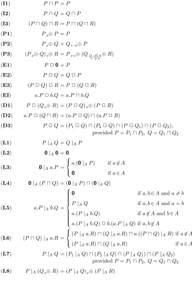
P ::=0 _{| a.P | P ⊓P | P} 2P | P |AP | Pp⊕P The intuitive meaning of the various constructs is straightforward:

(i) 0 _{represents the stopped process.}

(ii) a.P, whereais inAct, is a process which first performs the actiona, and then proceeds as P.

(iii) P ⊓Qis theinternal choice between the processesP andQ; it will act either like P or like Q, but a user is unable to influence which.

(iv) P 2Q is theexternal choice betweenP and Q; again it will act either like P or like Q but, in this case, according to the demands of a user.

(v) P |A Q, where A is a subset of Act, represents processes P and Q running in parallel. They may synchronise by performing the same action from A simultaneously; such a synchronisation results in an internal action τ 6∈ Act. In additionP and Q may independently do any action from (Act\A)∪ {τ}. (vi) Pp⊕Q, where p is an arbitrary probability, a real number strictly between 0

We usepCSPto denote the set of terms defined by this grammar, andCSPdenotes the subset of that which does not use the probabilistic choice. Of course the lan-guage CSP in all its glory [BHR84,Hoa85,OH86] has many more operators; we have simply chosen a representative selection, adding probabilistic choice to obtain an elementary probabilistic version of CSP. Our parallel operator is not a CSP prim-itive, but it can easily be expressed in terms of the CSP primitives—in particular P |A Q = (PkAQ)\A, where kA and \A are the parallel composition and hiding operators of [OH86]. It can also be expressed in terms of the parallel composition, renaming and restriction operators of CCS. We have chosen this (non-associative) operator for its convenience in defining the application of tests to processes.

As usual we tend to omit occurrences of 0_{; the action prefixing operator a.}

binds stronger than any of the binary operators, and precedence between the binary operators will be indicated via brackets or spacing. We will also sometimes usen-ary versions of the binary operators, such asL

i∈IpiPi withPi∈Ipi= 1, and ei∈IPi.

3.2 Operational Semantics of pCSP

The above intuitive reading of the various operators can be formalised by an op-erational semantics which associates with each process term a graph-like structure representing the manner in which it may react to users’ requests. Let us briefly recall this procedure for (non-probabilistic)CSP.

Definition 3.1 A labelled transition system (LTS) is a triple hS,Actτ,→i, where (i) S is a set of states

(ii) Actτ is a set of actionsAct, augmented with a new action symbolτ to represent synchronisations, and more generally internal unobservable activity

(iii) → ⊆ S×Actτ ×S represents the effect of performing actions.

It is usual to use the more intuitive notation s−→α s′ instead of (s, α, s′)∈ →. The operational semantics of CSP is obtained by endowing the set of terms with the structure of an LTS. Specifically

(i) the set of statesS is taken to be all terms from the languageCSP

(ii) the action relations P −→α Qare defined inductively on the syntax of terms. A precise definition may be found in [OH86].

In order to interpret the full pCSP operationally we need to generalise the notion of LTS to take probabilities into account. First we need some notation for probability distributions. A (discrete) probability distribution over a set S is a mapping ∆ :S →[0,1] with P

s∈S∆(s) = 1. The support of ∆ is given by

⌈∆⌉ := {s ∈ S | ∆(s) > 0}. For our simple setting we only require distribu-tions with finite support; letD(S), ranged over by ∆,Θ,Φ, denote the collection of all such distributions overS. We usesto denote the point distribution, satisfying

s(t) =

(

while if pi ≥0 and ∆i is a distribution for each i in some finite index set I, then

P

i∈Ipi·∆i is given by (X

i∈I

pi·∆i)(s) =

X

i∈I

pi·∆i(s)

If P

i∈Ipi = 1 then this is easily seen to be a distribution in D(S), and we will sometimes write it asp₁·∆1+. . .+pn·∆n when the index set I is{1, . . . , n}.

We can now present the probabilistic generalisation of an LTS:

Definition 3.2 A probabilistic labelled transition system (pLTS) is a triple

hS,Actτ,→i, where (i) S is a set of states

(ii) Actτ is a set of actionsAct, augmented by a new action τ, as above (iii) → ⊆ S×Actτ × D(S).

As with LTSs, we usually writes−→α ∆ in place of (s, α,∆)∈ →. An LTS may be viewed as a degenerate pLTS, one in which only point distributions are used. We now mimic the operational interpretation ofCSPas an LTS by associating with

pCSPa particular pLTShSp,Actτ,→i. However there are two major differences: (i) only a subset of terms inpCSPwill be used as the set of statesSp in the pLTS (ii) terms in pCSP will be interpreted as distributions over Sp, rather than as

elements of Sp.

First we define the subsetSp of states that we use: it is the least set satisfying (i) 0_∈Sp

(ii) a.P ∈Sp (iii) P ⊓Q∈Sp

(iv) s₁, s₂ ∈Sp impliess1 2s2 ∈Sp (v) s₁, s₂ ∈Sp impliess1 |As2∈Sp.

Thus,Spis the set ofpCSPexpressions in which every occurrence of the probabilistic choice operatorp⊕is weakly guarded, i.e. is within a subexpression of the form a.P or P ⊓ Q. The interpretation of terms in pCSP as distributions in D(Sp) is as follows:

(i) [0℄=0

(ii) [a.P℄=a.P

(iii) [P ⊓Q℄=P ⊓Q

(iv) [P

p⊕Q℄=p·[P℄+ (1−p)·[Q℄

(v) [P 2Q℄=[P℄2[Q℄

(vi) [P |AQ℄=[P℄|A[Q℄.

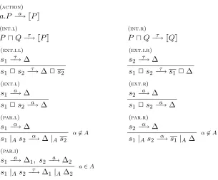
(action₎

a.P −→a [P℄

(int.l)

P ⊓Q−→τ [P℄

(int.r)

P ⊓Q−→τ [Q℄

(ext.i.l)

s1 −→τ ∆

s1 2s2 −→τ ∆2s2

(ext.i.r)

s2 −→τ ∆

s1 2s2 −→τ s12∆ (ext.l₎

s1 −→a ∆ s1 2s2 −→a ∆

(ext.r₎

s2 −→a ∆ s1 2s2 −→a ∆ (par.l₎

s₁ −→α ∆

s1 |As2−→α ∆|As2 α6∈A

(par.r₎

s₂ −→α ∆

s1 |As2 −→α s1 |A∆ α6∈A

(par.i)

s1 −→a ∆1, s2 −→a ∆2 s₁ |As2−→τ ∆1 |A∆2

a∈A

Fig. 1. Operational semantics ofpCSP. Herearanges overActandαoverActτ.

as binary operators over Sp, and can therefore be lifted to D(Sp) in the standard manner. Namely we define

(∆12∆2)(s) =

(

∆1(t1)·∆2(t2) ifs=t12t2,

0 otherwise

with ∆1 |A∆2 given similarly; note that as a result we have[P℄=P for allP∈Sp.

Finally the definition of the relations−→α is given in Figure 1. These rules are very similar to the standard ones used to interpretCSP as an LTS [OH86], modified to take into account that the result of an action must be a distribution. For example (int.l) and (int.r) say that P ⊓Q makes an internal unobservable choice to act

either like P or like Q. Similarly the four rules (ext.l), (ext.r), (ext.i.l) and

(ext.i.r) can be read as giving the standard interpretation to the external choice

operator: the processP 2_{Qmay perform any external action of its componentsP}

andQ, which resolves the choice; it may also perform any of their internal actions, but when these are performed the choice is not resolved.

3.3 The precedence of probabilistic choice

Our operational semantics entails that2_{and|Adistribute over probabilistic choice:}

[P 2(Qp⊕R)℄ =[(P 2Q)

p⊕(P 2R)℄ [P |A(Qp⊕R)℄ =[(P |AQ)

In Section 6.5, these identities will return as axioms of may testing. However, this is not so much a consequence of our testing methodology: it is hardwired in our interpretation[ ℄ofpCSPexpressions as distributions. We could have obtained the

same effect by introducingpCSPas a two-sorted language, given by the grammar P::=S | Pp⊕P

S::=0 _{| a.P | P ⊓P | S} 2S | S |AS

and introducing expressions like P 2 _{(Qp⊕ R) and P |A (Qp⊕ R) as syntactic}

sugar for the grammatically correct expressions obtained by distributing2 _{and |A}

overp⊕. In that case, theS-expressions would constitute the setSp of states in the pLTS of pCSP, and [s℄=sfor any s∈Sp.

A consequence of our operational semantics is that in the processa.(b1

2⊕c)|∅ d the action d can be scheduled either beforea, or after the probabilistic choice be-tween b and c—but it can not be scheduled after a and before this probabilistic choice. We justify this by thinking ofPp⊕Qnot as a process that starts with mak-ing a probabilistic choice, but rather as one thathas just made such a choice, and with probabilitypis no more and no less than the process P. Thusa.(Pp⊕Q) is a process that in doing thea-step makes a probabilistic choice between the alternative targetsP andQ.

This design decision is in full agreement with previous work featuring nondeter-minism, probabilistic choice and parallel composition [HJ90,WL92,Seg95]. More-over, a probabilistic choice between processesP andQthat does not take precedence over actions scheduled in parallel can simply be written asτ.(Pp⊕Q). Here τ.P is an abbreviation for P ⊓P. Using the operational semantics of ⊓ in Figure1, τ.P is a process whose sole initial transition isτ.P −→τ P, henceτ.(Pp⊕Q) is a process that starts with making a probabilistic choice, modelled as an internal action, and with probabilitypproceeds asP. Any activity scheduled in parallel withτ.(Pp⊕Q) can now be scheduled before or after this internal action, hence before or after the making of the choice. In particular,a.τ.(b1

2⊕c)|∅ d allowsd to happen between a and the probabilistic choice.

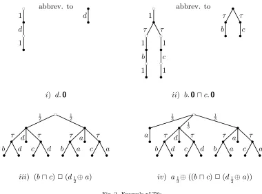
3.4 Graphical representation of pCSPprocesses

We graphically depict the operational semantics of apCSPexpression P by drawing the part of the pLTS defined above that is reachable from [P℄ as a finite acyclic

b c b 1 b c d b 1

abbrev. to b b d b c b 1 b c τ b 1 b c b b 1 b c τ b 1 b c c b 1

abbrev. to b b τ b b b τ b c

i) d.0 _{ii) b.}0_⊓c.0

b c b 1 2 b τ b b b d b d b τ b c b d b 1 2 b τ b b b a b a b τ b c b a b c b 1 3 b a

b 13

b τ b b b d b d b τ b c b d b 1 3 b τ b b b a b a b τ b c b a

iii) (b⊓c)2_(d1

2⊕a) iv) a13⊕((b⊓c)

2_(d1 2⊕a))

Fig. 2. Example pLTSs from top to bottom.

A few examples are described in Figure 2. In i) we find [d.0℄ as the point

distributiond.0_{, represented by a tree with one edge from the root, labelled with}

the probability 1, to the state d.0_{. In turn this state is represented as the subtree}

with one outgoing edge, labelled by the only possible action dto [0℄. Finally this

is also a point distribution, represented as a subtree with one edge leading to a leaf, labelled by the probability 1.

These edges labelled by probability 1 occur so frequently that it makes sense to omit them, together with the associated nodes ◦ representing point distributions. With this convention [d.0℄ turns out to be a simple tree with one edge labelled

by the action d. The same convention simplifies considerably the representation of b ⊓ c in ii), resulting in an LTS detailing an internal choice between the two actions. Officially, the endnodes of this graph ought to be merged, as both of them represent the process0_{. However, for reasons of clarity, in graphical representations}

we often unwind the underlying graph into a tree, thus representing the same state or distribution multiple times.

The interpretation of (b⊓c)2_(d1

2⊕a) is more interesting. This requires clause (v) above in the definition of[ ℄, resulting in the distribution (b⊓c)2∆, where ∆

is the distribution resulting from the interpretation of (d1

2⊕ a), itself a two-point distribution mapping both the statesd.0 _{and a.}0 _{to the probability} 1

2. The result is again a two-point distribution, this time mapping the two states (b ⊓ c) 2 _d

(a.ω1

4⊕(b2c.ω))|Act(b2c2d)

a.ω|Act(b2c2d) 1 4

(b2_c.ω)|Act(b2c2_d)

3 4

0|Act0 τ

ω |Act0 τ

0|Act0 ω

Apply((a.ω1

4⊕(b2c.ω)),(b2c2d)) = 1

4· {0}+34 · {0,1}={0,34} Fig. 3. Example of testing

representation which results when this term is combined probabilistically with the simple processa.0_.

To sum up, the operational semantics endows pCSP with the structure of a pLTS, and the function[ ℄interprets process terms inpCSPas distributions in this

pLTS, which can be represented by finite acyclic directed graphs (typically drawn as trees), with edges labelled either by probabilities or actions, so that edges labelled by actions and probabilities alternate (although in pictures we may suppress 1-labelled edges and point distributions).

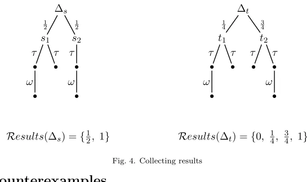
3.5 Testing pCSPprocesses

Let us now turn to applying the testing theory from Section 2 to pCSP. As with the standard theory [DH84,Hen88], we use as tests any process from pCSP itself, which in addition can use a special symbol ω to report success. For example, a.ω1

4⊕(b2c.ω) is a probabilistic test, which 25% of the time requests anaaction, and 75% requests that ccan be performed. If it is used as must test the 75% that requests acaction additionally requires thatbis not possible. As in [DH84,Hen88], it is not the execution ofω that constitutes success, but the arrival in a state where ω is possible. The introduction of the ω-action is simply a method of defining a success predicate on states without having to enrich the language of processes explicitly with such predicates.

Formally, letω6∈Actτ and writeActω forAct∪ {ω}andActωτ forAct∪ {τ, ω}. In Figure1 we now let arange over Actω and α over Actω_τ. Tests may have subterms ω.P, but other processes may not. To apply the testT to the processP we run them in parallel, tightly synchronised; that is, we run the combined processT |ActP. Here P can only synchronise withT, and in turn the testT can only perform the success actionω, in addition to synchronising with the process being tested; of course both tester and testee can also perform internal actions. An example is provided in Figure 3, where the test a.ω1

see that 25% of the time the test is unsuccessful, in that it does not reach a state where ω is possible, and 75% of the time itmay be successful, depending on how the now internal choice between the actions b and c is resolved, but it is not the case that itmust be successful.

[T |Act P℄ is representable as a finite graph which encodes all possible

interac-tions of the testT with the process P. It only contains the actions τ and ω. Each occurrence of τ represents a nondeterministic choice, either in T or P themselves, or as a nondeterministic response byP to a request fromT, while the distributions represent the resolution of underlying probabilities inT andP. We use the structure

[T |ActP℄ to defineApply(T, P), the non-empty finite subset of [0,1] representing

the set of probabilities that applyingT to P will be a success.

First we define a function Results( ), which when applied to any state in Sp returns a finite subset of [0,1]. The definition will require that it be also applied to distributions, and to do so we need to usechoice functions for collecting elements from subsets of [0,1]. Suppose R :Sp → P_fin+([0,1]), and c : X → [0,1], where X is a subset of Sp. Then we write c∈XR if c(s)∈R(s) for every s in X, and the results-collecting function can be defined as follows:

Results(s) =

  

 

{1} ifs−→ω ,

S

{ Results(∆) | s−→τ ∆} ifs6−−→ω, s−→τ ,

{0} otherwise

where

Results(∆) = { X

s∈⌈∆⌉

∆(s)·c(s) | c∈_⌈∆⌉Results}

However, instead of the explicit use of choice functions, we will tend to use the more convenient notation

Results(∆) = ∆(s1)· Results(s1) +. . .+ ∆(sn)· Results(sn)

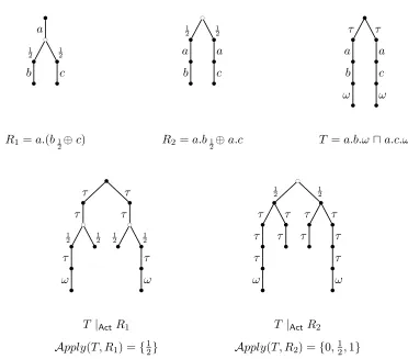
where ⌈∆⌉ = {s1, . . . sn}. Note that Results( ) is indeed a well-defined function, because the pLTShSp,Actτ,→iis finitely branching and well-founded.

For example consider the transition systems in Figure4, where for reference we have labelled the nodes. ThenResults(s1) = {1,0} while Results(s2) = {1}, and thereforeResults(∆s) = 1₂· {1,0}+1₂· {1} which, since there are only two possible choice functionsc∈⌈∆s⌉Results, evaluates further to {12,1}. Similarly Results(t1) = Results(t2) = {0,1} and using the four choice functions c∈⌈∆t⌉Results, the

calculation ofResults(∆t) = 1₄· {0,1}+3₄ · {0,1} leads to {0,1₄,3₄,1}.

Definition 3.3 For anyP∈pCSPandT∈ T letApply(T, P) =Results([T|ActP℄).

With this definition we now have two testing preorders forpCSP, one based onmay

∆s s1

1 2

b τ

b ω

b τ

s2 1 2

b τ

b ω

∆t t1

1 4

b τ

b ω

b τ

t2 3 4

b τ

b τ

b ω

Results(∆s) ={1₂, 1} Results(∆t) ={0, 1₄, 3₄, 1}

Fig. 4. Collecting results

4

Counterexamples

We will see in this section that many of the standard testing axioms are not valid in the presence of probabilistic choice. We also provide counterexamples for a few distributive laws involving probabilistic choice that may appear plausible at first sight. In all cases we establish a statement P 6≃_pmay Q by exhibiting a test T such that max(Apply(T, P)) 6= max(Apply(T, Q)) and a statement P 6≃_pmust Q by exhibiting a test T such that min(Apply(T, P)) 6= min(Apply(T, Q)). In case

max(Apply(T, P))>max(Apply(T, Q)) we find in particular thatP 6⊑_pmay Q, and in casemin(Apply(T, P))>min(Apply(T, Q)) we obtain P 6⊑_pmust Q.

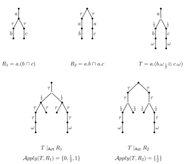
Example 4.1 The axioma.(Pp⊕Q) =a.Pp⊕a.Qis unsound.

Consider the example in Figure 5. In R1 the probabilistic choice between b and c is taken after the action a, while in R2 the choice is made before the action has happened. These processes can be distinguished by the nondeterministic test T = a.b.ω⊓a.c.ω. First consider running this test onR₁. There is an immediate choice made by the test, effectively running either the testa.b.ωon R1 or the testa.c.ω; in fact the effect of running either test is exactly the same. Considera.b.ω. When run onR1theaaction immediately happens, and there is a probabilistic choice between runningb.ω on eitherb orc, giving as possible results{1} or {0}; combining these according to the definition of the functionResults( ) we get 1₂· {0}+₂1· {1}={1₂}. Since running the test a.c.ω has the same effect, Apply(T, R1) turns out to be the same set{1₂}.

Now consider running the test T on R₂. Because R₂, and hence also T |ActR2, starts with a probabilistic choice, due to the definition of the function Results( ), the test must first be applied to the probabilistic components,a.b and a.c, respec-tively, and the results subsequently combined probabilistically. When the test is run ona.b, immediately a nondeterministic choice is made in the test, to run either a.b.ωora.c.ω. With the former we get the result{1}, with the latter{0}, so overall, for runningT on a.b, we get the possible results{0,1}. The same is true when we run it ona.c, and therefore Apply(T, R2) = 1₂ · {0,1}+₂1 · {0,1}={0,1₂,1}.

b b c a b 1 2 b b b 1 2 b c b c b 1 2 b a b b b 1 2 b a b c b b τ b a b b b ω b τ b a b c b ω

R₁ =a.(b1

2⊕c) R2 =a.b12⊕a.c T =a.b.ω ⊓a.c.ω b b τ b c τ b 1 2 b τ b ω b 1 2 b τ b c τ b 1 2 b 1 2 b τ b ω b c b 1 2 b τ b τ b τ b ω b τ b τ b 1 2 b τ b τ b τ b τ b τ b ω

T |ActR1 T |ActR2

Apply(T, R1) ={1₂} Apply(T, R2) ={0,1₂,1} Fig. 5. Counterexample: action prefix does not distribute over probabilistic choice

Example 4.2 The axioma.(P ⊓Q) =a.P ⊓a.Q is unsound.

It is well known that this axiom is valid in the standard theory of testing, for non-probabilistic processes. However, consider the instanceR1 and R2 in Figure6, and note that these processes do not contain any probabilistic choice. But they can be differentiated by the probabilistic testT =a.(b.ω1

2⊕c.ω); the details are in Figure6. There is only one possible outcome from applyingTtoR2, the probability 1₂, because the nondeterministic choice is made before the probabilistic choice. On the other hand whenT is applied toR₁there are three possible outcomes, 0, 1₂ and 1, because effectively the probabilistic choice takes precedence over the nondeterministic choice. So we haveR₁6⊑_pmay R₂ andR₂ 6⊑_pmust R₁.

Example 4.3 The axioma.(P 2_{Q) =}a.P 2a.Q is unsound.

This axiom is valid in the standard may-testing semantics. However, consider the two processes R₁ = a.(b 2 _c), R₂ = a.b 2 a.c and the probabilistic test T = a.(b.ω 1

2⊕ c.ω). Now Apply(T, R1) = {1} and Apply(T, R2) ={ 1

b b a b τ b b b τ b c b b τ b a b b b τ b a b c b b c a b 1 2 b b b ω b 1 2 b c b ω

R₁=a.(b⊓c) R₂ =a.b⊓a.c T =a.(b.ω1 2⊕c.ω)

b b c τ b 1 2 b τ b τ b ω b τ b 1 2 b τ b τ b τ b ω b b τ b c τ b 1 2 b τ b ω b 1 2 b τ b c τ b 1 2 b 1 2 b τ b ω

T |ActR1 T |ActR2

Apply(T, R1) ={0,1₂,1} Apply(T, R2) ={1₂} Fig. 6. Counterexample: action prefix does not distribute over internal choice

Example 4.4 The axiomP =P 2P is unsound. Let R1, R2 denote (a 1

2⊕ b) and (a 12⊕ b)

2 _(a 1

2⊕ b), respectively. It is easy to calculate that Apply(a.ω, R1) ={1₂} but, because of the way we interpret exter-nal choice as an operator over distributions of states in a pLTS, it turns out that

[R2℄=[((a2a)1

2⊕(a2b))12⊕((b2a)12⊕(b2b))

℄and soApply(a.ω, R2) ={

3 4}. ThereforeR2 6⊑pmayR1 and R2 6⊑pmust R1.

Example 4.5 The axiomPp⊕(Q⊓R) = (Pp⊕Q)⊓(Pp⊕R) is unsound. Consider the processes R₁ = a1

2⊕ (b ⊓c) and R2 = (a21⊕b) ⊓ (a12⊕c), and the test T1 = a.ω ⊓ (b.ω 1

2⊕ c.ω). In the best of possible worlds, when we apply T1 to R1 we obtain probability 1, that is max(Apply(T1, R1)) = 1. Informally this is because half the time when it is applied to the subprocess a of R1, optimistically the sub-testa.ω is actually run. The other half of the time, when it is applied to the subprocess (b ⊓ c), optimistically the sub-test Tr = (b.ω 1

Apply(T1, R1) = 1₂ · Apply(T1, a) + 1₂· Apply(T1, b⊓c) = 1₂ ·(Apply(a.ω, a)∪ Apply(Tr, a)) +

1

2·(Apply(T1, b)∪ Apply(T1, c)∪ Apply(a.ω, b⊓c)∪ Apply(Tr, b⊓c)) = 1₂ ·({1} ∪ {0}) +1₂ ·({0,1₂} ∪ {0,1₂} ∪ {0} ∪ {0,1₂,1})

={0,1₄,1₂,3₄,1}

However no matter how optimistic we are when applyingT1 toR2 we can never get probability 1; the most we can hope for is 3₄, which might occur when T₁ is applied to the subprocess (a1

2⊕b). Specifically when the subprocess ais being tested the sub-testa.ωmight be used, giving probability 1, and when the subprocessbis being tested the sub-test (b.ω1

2⊕c.ω) might be used, giving probability 1

2. We leave the reader to check that formally

Apply(T1, R2) ={0,1₄,1₂,3₄} from which we can concludeR1 6⊑pmay R2.

We can also show that R26⊑pmust R1, using the test T2 = (b.ω2c.ω)⊓(a.ω1

3⊕(b.ω12⊕c.ω)).

Reasoning pessimistically, the worst that can happen when applyingT2 toR1 is we get probability 0. Each time the subprocess a is tested the worst probability will occur when the sub-test (b.ω2_{c.ω) is used; this results in probability 0. Similarly}

when the subprocess (b ⊓c) is being tested the subtest (a.ω1

3⊕(b.ω12⊕c.ω)) will give probability 0. In other words min(Apply(T2, R1)) = 0. When applying T2 to R2, things can never be as bad. The worst probability will occur whenT2 is applied to the subprocess (a1

2⊕b), namely probability 1

6. We leave the reader to check that formallyApply(T2, R1) ={0,₆1,1₃,1₂,2₃}and Apply(T2, R2) ={1₆,1₃,1₂,2₃}.

Example 4.6 The axiomP ⊓(Qp⊕R) = (P ⊓Q)p⊕(P ⊓R) is unsound. LetR1 =a⊓(b1

2⊕c),R2 = (a⊓b)12⊕(a⊓c) and T =a.(ω12⊕0)2b.ω. One can check thatApply(T, R1) ={1₂} and Apply(T, R2) = 1₂{1₂,1}+ 1₂{1₂,0}={1₄,1₂,3₄}. Therefore we have R2 6⊑pmay R1 and R1 6⊑pmustR2.

Example 4.7 The axiomP 2_{(Q⊓R) = (P} 2_Q)⊓(P 2_{R) is unsound.}

Let R₁ = (a 1

2⊕ b) 2 (c ⊓ d), R2 = ((a 12⊕ b) 2 c) ⊓ ((a 12⊕ b) 2 d) and T = (a.ω 1

2⊕c.ω) ⊓ (b.ω12⊕ d.ω). This time we get Apply(T, R1) = {0, 1

4,12,34,1} andApply(T, R2) ={1₄,3₄}. SoR16⊑pmay R2 andR2 6⊑pmust R1.

Example 4.8 The axiomP ⊓(Q2_{R) = (P ⊓Q)}2_{(P ⊓R) is unsound.}

LetR1 = (a1

2⊕b)⊓((a12⊕b)2

0_{) andR2 = ((a}1

2⊕b)⊓(a12⊕b))2((a12⊕b)⊓

0_).

One obtainsApply(a.ω, R1) ={1₂} and Apply(a.ω, R2) ={1₂,3₄}. So R2 6⊑pmay R1. LetR₃ and R₄ result from substitutinga1

Example 4.9 The axiomPp⊕(Q2R) = (Pp⊕Q)2(Pp⊕R) is unsound. Let R1 = a1

2⊕ (b

2 _{c), R2 = (a}1 2⊕ b)

2 _(a1

2⊕ c) and R3 = (a

2 _b)1 2⊕ (a

2 _c).

R₁ is an instance of the left-hand side of the axiom, andR₂an instance of the right-hand side. Here we useR3 as a tool to reason aboutR2, but in Section8we needR3 in its own right. Note that[R2℄=

1

2·[R1℄+

1

2·[R3℄. LetT =a.ω. It is easy to see

thatApply(T, R1) ={1₂} and Apply(T, R3) ={1}. ThereforeApply(T, R2) ={3₄}. So we haveR26⊑pmay R1 andR2 6⊑pmust R1.

Of all the examples in this section, this is the only one for which we can show that ⊑pmay and ⊒pmay both fail, i.e. both inequations that can be associated with the axiom are unsound formay testing. LetT =a.(ω 1

2⊕

0_{) ⊓(b.ω}1

2⊕c.ω). It is not hard to check thatApply(T, R1) ={0,1₄,1₂,3₄} and Apply(T, R3) ={1₂}. Thus

Apply(T, R2) ={1₄,3₈,1₂,5₈}. Therefore, we have R1 6⊑pmay R2.

For future reference, we also observe that R16⊑pmay R3 andR36⊑pmay R1.

5

Must versus may testing

OnpCSPthere are two differences between the preorders⊑pmay and ⊑pmust:

• _{Must testing is more discriminating}

• _{The preorders ⊑pmay and ⊑pmust are oriented in opposite directions.}

In this section we substantiate these claims by proving that P ⊑pmust Q implies Q⊑pmayP, and by providing a counterexample that shows the implication is strict. We are only able to obtain the implication since our language does not feature di-vergence, infinite sequences ofτ-actions. It is well known from the non-probabilistic theory of testing [DH84,Hen88] that in the presence of divergence≃may and ≃must are incomparable.

To establish a relationship between must testing and may testing, we define the context C[ ] = |{ω} (ω 2 (ν ⊓ν)) so that for every test T we obtain a new test

C[T], by considering ν instead ofω as success action.

Lemma 5.1 For any processP and test T, it holds that (i) ifp∈ Apply(T, P) then (1−p)∈ Apply(C[T], P)

(ii) if p∈ Apply(C[T], P) then there exists a q∈ Apply(T, P) such that 1−q ≤p.

Proof. A state of the form C[s]|Act tcan always do a τ-move, and never directly a success action ν. The τ-steps that C[s] |Act t can do fall into three classes: the resulting distribution is either

• _{a point distribution v with v −→}ν _{; we call this a successful τ-step, because it}

contributes 1 to the set Results(C[s]|Actt)

• _{a point distribution u with u a state from which the success action ν is}

un-reachable; we call this anunsuccessful τ-step, because it contributes 0 to the set

Results(C[s]|Actt)

Note that

• _{C[s]|Acttcan always do a successfulτ-step}

• _{C[s]|Acttcan do an unsuccessfulτ-step iff s|Act tcan do aω-step} • _{and C[s]|Actt−→}τ _{C[Θ]|Act∆ iffs|Actt−→}τ _Θ|Act∆.

Using this, both claims follow by a straightforward induction onT and P. 2

Proposition 5.2 IfP ⊑pmust QthenQ⊑pmayP.

Proof. SupposeP ⊑pmustQ. We must show that, for any testT, ifp∈ Apply(T, Q) then there exists a q ∈ Apply(T, P) such that p≤q. So supposep ∈ Apply(T, Q). By the first clause of Lemma 5.1, we have (1−p) ∈ Apply(C[T], Q). Given that P ⊑pmust Q, there must be an x ∈ Apply(C[T], P) such that x ≤ 1−p. By the second clause of Lemma5.1, there exists aq ∈ Apply(T, P) such that 1−q ≤x. It

follows thatp≤q. ThereforeQ⊑pmay P. 2

Example 5.3 To show that must testing is strictly more discriminating than may testing consider the processesa2banda⊓b, and expose them to testa.ω. It is not hard to see thatApply(a.ω, a2_{b) ={1}, whereasApply(a.ω, a⊓b) ={0,1}. Since}

min(Apply(a.ω, a2_{b)) = 1 and min(Apply(a.ω, a⊓b)) = 0, using Proposition 2.1}

we obtain that (a2b)6⊑_pmust (a⊓b).

Since max(Apply(a.ω, a 2 _{b)) =} max(Apply(a.ω, a ⊓ b)) = 1, as a may test, the test a.ω does not differentiate between a 2 _{b and a ⊓ b. In fact, we have}

(a⊓b)⊑pmay (a2b), and even (a2b)≃pmay (a⊓b), but this cannot be shown so easily, as we would have to consider all possible tests. In Section6 we will develop a tool to prove statements P ⊑pmay Q, and apply it to derive the equality above (axiom (EI) in Figure8).

6

Simulations

The examples of Section 4 have been all negative, because one can easily demon-strate an inequivalence between two processes by exhibiting a test which distin-guishes them in the appropriate manner. A direct application of the definition of the testing preorders is usually unsuitable for establishing positive results, as this involves a universal quantification over all possible tests that can be applied. To give positive results of the form P ⊑pmay Q (and similarly for P ⊑pmust Q) we need to come up with a preorder⊑finer such that (P ⊑finerQ)⇒(P ⊑pmayQ) and statementsP ⊑finerQ can be obtained by exhibiting a single witness.

In this section we report on investigations in this direction, usingsimulations as our witnesses. We confine ourselves tomay testing, although similar results hold for

6.1 Lifting relations

LetR ⊆S× D(S) be a relation from states to distributions. We lift it to a relation

R ⊆ D(S)× D(S) by letting ∆1R∆2 whenever

(i) ∆1 =Pi∈Ipi·si, whereI is a finite index set and

P

i∈Ipi= 1 (ii) For each i∈I there is a distribution Φi such thatsi RΦi (iii) ∆2 =Pi∈Ipi·Φi.

An important point here is that in the decomposition (i) of ∆1 intoPi∈Ipi·si, the states si are not necessarily distinct: that is, the decomposition is not in general unique. Thus when establishing the relationship between ∆1 and ∆2, a given state s in ∆1 may play a number of different roles, and this is seen clearly if we apply this definition to the action relations−→ ⊆α Sp× D(Sp) in the operational semantics of pCSP. We obtain lifted relations between D(Sp) and D(Sp), which to ease the notation we write as ∆1 −→α ∆2; then, usingpCSPterms to represent distributions, a simple instance of a transition between distributions is given by

(a.b2a.c)1 2⊕a.d

a

−→ b1

2⊕d

But we also have

(a.b2_a.c)1 2⊕a.d

a

−→ (b1

2⊕c)12⊕d (1) because, viewed as a distribution, the term (a.b2_a.c)1

2⊕a.dmay be re-written as ((a.b2_a.c)1

2⊕(a.b

2_a.c)) 1

2⊕ a.d representing the sum of point distributions 1

4 ·(a.b2a.c) + 14·(a.b2a.c) +12 ·a.d

from which the move (1) can easily be derived using the three moves from states a.b2a.c−→a b a.b2a.c−→a c a.d−→a d

The lifting construction satisfies the following two useful properties, whose proofs we leave to the reader.

Proposition 6.1 SupposeR ⊆S× D(S) and P

i∈Ipi = 1. Then we have (i) Θi R∆i implies (P

i∈Ipi·Θi)R(Pi∈Ipi·∆i). (ii) If (P

i∈Ipi·Θi) R ∆ then ∆ = Pi∈Ipi·∆i for some set of distributions ∆i

such that Θi R∆i. 2

terms to denote distributions, we have (a⊓b)1

2⊕(a⊓c) ˆ τ

−→ a1

2⊕(a⊓b 12⊕ c) This follows because as a distribution (a⊓b)1

2⊕(a⊓c) may be written as 1

4 ·(a⊓b) +14 ·(a⊓b) +14 ·(a⊓c) +14 ·(a⊓c) and we have the four moves from states to distributions:

(a⊓b)−→τˆ a (a⊓b)−→τˆ (a⊓b) (a⊓c)−→τˆ a (a⊓c)−→τˆ c

6.2 The simulation preorder

Following tradition it would be natural to define simulations as relations between states in a pLTS [JWL01,SL94]. However, technically it is more convenient to use relations in Sp ↔ D(Sp). One reason may be understood through the example in Figure 5. Although in Example 4.1 we found that R2 6⊑pmay R1, we do have R₁ ⊑pmayR2. If we are to relate these processes via a simulation-like relation, then the initial state ofR1 needs to be related to the initialdistributionofR2, containing the two statesa.b and a.c.

Our definition of simulation uses weak transitions [Mil89], which have the stan-dard definitions except that they now apply to distributions, and−→τˆ is used instead of−→τ . This reflects the understanding that if a distribution may perform a sequence of internal moves before or after executing a visible action, different parts of the distribution may perform different numbers of internal actions:

• _{Let ∆1 =}τ_⇒ˆ _{∆2 whenever ∆1 −→}τˆ ∗_∆2.

• _{Similarly ∆1 =⇒}ˆa _{∆2 denotes ∆1 −→}τˆ ∗_−→a _−→τˆ ∗_{∆2 whenever} a∈Act.

Definition 6.2 [Seg95] A relation R ⊆Sp× D(Sp) is said to be asimulation if for all s,∆, α,Θ we have that s R ∆ and s −→α Θ implies there exists some ∆′ with ∆=α⇒ˆ ∆′ and ΘR∆′.

We write s

S ∆ to mean that there is some simulation R such that sR ∆. Note that the lifting operation on relations ismonotone, in the sense that R ⊆ Simplies

R ⊆ S. Hence

S, which is the union of all simulations, is a simulation itself. Therefore,

S could just as well have been defined co-inductively as the largest relation _S⊆Sp× D(Sp) satisfying, for all s∈Sp, ∆∈ D(Sp) and α∈Actτ,

sR∆∧s−→α Θ ⇒ ∃∆′.∆=α⇒ˆ ∆′∧ΘR∆′

Definition 6.3 The simulation preorder on process terms is defined by letting P ⊑S Q whenever there is a distribution ∆ with [Q℄

ˆ τ

=⇒ ∆ and [P℄

s0 ∆1 a

s1 1 2

b b

s2 1 4

b c

s3 1 4

b c

t0 ∆2 a

t1 1 4

b b

t2 1 4

b b

t3 1 2

b c

P1 =a.(b1

2⊕(c12⊕c)) P2 =a.((b12⊕b)12⊕c) Fig. 7. Two simulation equivalent processes

If P ∈ Sp, that is if P is a state in the pLTS of pCSP and so [P℄ = P, then to

establish P ⊑S Q it is sufficient to exhibit a simulation between the state P and the distribution[Q℄, because triviallys

S ∆ impliessS ∆.

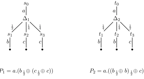
Example 6.4 Consider the two processes Pi in Figure 7. To show P1 ⊑S P2 it is sufficient to exhibit a simulation R such that s0 R t0. Let R ⊆ Sp× D(Sp) be defined by

s₀ R t₀ s₁ R ∆t s₂ R t₃ s₃ R t₃ 0 _R 0

where ∆tis the two-point distribution mapping botht1 andt2 to the probability 1₂. Then it is straightforward to check that it satisfies the requirements of a simulation: the only non-trivial requirement is that ∆1 R ∆2. But this follows from the fact that

∆1 = 1₂ ·s1+₄1 ·s2+1₄ ·s3 ∆2 = 1₂ ·∆t+ 1₄·t3+1₄ ·t3 As another example reconsiderR1=a.(b1

2⊕c) andR2 =a.b12⊕a.cfrom Figure 5, where for convenience we use process terms to denote their semantic interpretations. It is easy to see thatR1 ⊑SR2 because of the simulation

R1 R [R2℄ b R b c R c 0 R 0

Namely R₂ −→a (b1

2⊕c) and (b12⊕c)R(b12⊕c). Similarly (a1

2⊕ c) ⊓ (b12⊕c) ⊑S (a ⊓ b)12⊕ c because it is possible to find a simulation between the state (a1

2⊕c)⊓(b12⊕c) and the distribution (a⊓b)12⊕c. In case P6∈Sp, a statement P ⊑S Q cannot always be established by a simulation

Rsuch that[P℄R[Q℄.

Example 6.5 Compare the processes P = a1

2⊕ b and P ⊓ P. Note that

[P℄ is

the distribution 1₂ a+1₂ b whereas [P ⊓ P℄ is the point distribution P ⊓P. The

relation Rgiven by

is a simulation, because theτ-stepP ⊓P −→τ (1₂ a+1₂ b) can be matched by the idle transition (₂1 a+1₂ b) =⇒ˆτ (1₂ a+₂1 b), and we have (1₂ a+1₂ b) R(1₂ a+1₂ b). Thus (P ⊓P)

S ( 1

2 a+12 b) =[P℄, hence[P ⊓P℄

S[P℄, and therefore P ⊓P ⊑SP.

This type of reasoning does not apply to the other direction. Any simulation

R with (1₂ a +1₂ b) R P ⊓P would have to satisfy a R P ⊓P and b R P ⊓P. However, the move a−→a 0 _{cannot be matched by the process P ⊓P, as the only}

transition the latter process can do is P ⊓P−→τ (1₂ a+1₂ b), and only half of that distribution can match the a-move. Thus, no such simulation exists, and we find

[P℄6

S [P ⊓P℄. Nevertheless, we still have P ⊑S P ⊓P. Here, the transition

ˆ τ =⇒

from Definition 6.3 comes to the rescue. As [P ⊓P℄

ˆ τ

=⇒ [P℄ and [P℄

S [P℄, we

obtain P ⊑SP ⊓P.

Because of the asymmetric use of distributions in the definition of simulation it is not immediately obvious that ⊑S is actually a preorder (a reflexive and transitive relation) and hence≃S an equivalence relation. In order to show this, we first need to establish some properties of

S.

Lemma 6.6 Suppose P

i∈Ipi = 1 and ∆i =⇒αˆ Φi for each i∈I, with I a finite index set. (Recall thatP

i∈Ipi·∆i is only defined for finite I.) Then

X

i∈I

pi·∆i =α⇒ˆ

X

i∈I pi·Φi

Proof. We first prove the case α = τ. For each i∈I there is a number ki such that ∆i = ∆i0 −→ˆτ ∆i1 −→τˆ ∆i2 −→ · · ·τˆ −→τˆ ∆iki = ∆′i. Let k = max{ki | i∈I}, using thatI is finite. Since we have Φ−→ˆτ Φ for any Φ∈ D(S), we can add spurious transitions to these sequences, until allki equalk. After this preparation the lemma follows byk applications of Proposition6.1(i), taking −→ˆτ forR.

The case α∈Actnow follows by one more application of Proposition6.1(i), this time withR=−→a , preceded and followed by an application of the case α=τ. 2

Lemma 6.7 Suppose ∆

SΦ and ∆ α

−→∆′. Then Φ=α⇒ˆ Φ′ for some Φ′ such that ∆′

SΦ

′_.

Proof. First ∆

SΦ means that

∆ =X

i∈I

pi·si, siS Φi, Φ =

X

i∈I

pi·Φi ; (2)

also ∆−→α ∆′ means

∆ =X

j∈J

qj·tj, tj −→α Θj, ∆′=X j∈J

qj ·Θj , (3)

and we can assumew.l.o.g. that all the coefficients pi, qj are non-zero. Now define Ij ={i∈I | si =tj} and Ji ={j∈J | tj =si},so that trivially

and note that

∆(si) =

X

j∈Ji

qj and ∆(tj) =

X

i∈Ij

pi (5)

Because of (5) we have

Φ =X i∈I

pi·Φi=

X

i∈I pi·

X

j∈Ji qj ∆(si) ·Φi

=X

i∈I

X

j∈Ji pi·qj ∆(si) ·Φi

Now for eachj in Ji we know that in fact tj =si, and so from the middle parts of (2) and (3) we obtain Φi =α⇒ˆ Φij such that Θj

SΦij. Lemma6.6 yields Φ=α⇒ˆ Φ′ =X

i∈I

X

j∈Ji pi·qj ∆(si)·Φij

where within the summationssi =tj, so that, using (4), Φ′ can also be written as

X

j∈J

X

i∈Ij pi·qj

∆(tj) ·Φij (6)

All that remains is to show that ∆′

SΦ

′_{,which we do by manipulating ∆}′ _{so that}

it takes on a form similar to that in (6): ∆′ =X

j∈J qj·Θj

=X

j∈J

qj·X

i∈Ij pi

∆(tj) ·Θj using (5) again

=X

j∈J

X

i∈Ij pi·qj ∆(tj)

·Θj

Comparing this with (6) above we see that the required result, ∆′

S Φ′, follows

from an application of Proposition6.1(i). 2

Lemma 6.8 Suppose ∆

SΦ and ∆ ˆ α

=⇒∆′. Then Φ=α⇒ˆ Φ′ for some Φ′ such that ∆′

SΦ

′_.

Proof. First we consider two claims (i) If ∆

SΦ and ∆ ˆ τ

−→∆′, then Φ=⇒ˆτ Φ′ for some Φ′ such that ∆′

SΦ

′_.

(ii) If ∆

SΦ and ∆ ˆ τ

=⇒∆′, then Φ=⇒ˆτ Φ′ for some Φ′ such that ∆′

SΦ

′_.

The proof of claim (i) is similar to the proof of Lemma6.7. Claim (ii) follows from claim (i) by induction on the length of the derivation of=τ⇒ˆ . By combining claim (ii)

Proposition 6.9 The relation

S is both reflexive and transitive on distributions.

Proof. We leave reflexivity to the reader; it relies on the fact thats

S sfor every state s.

For transitivity, let R ⊆Sp× D(Sp) be given by sRΦ iff s

S∆SΦ for some intermediate distribution ∆. Transitivity follows from the two claims

(i) Θ

S∆SΦ implies ΘRΦ (ii) R is a simulation, henceR ⊆

S.

Claim (ii) is a straightforward application of Lemma6.8, so let us look at (i). From

Θ

S∆ we have

Θ =X

i∈I

pi·si, si

S ∆i, ∆ =

X

i∈I pi·∆i

Since ∆

S Φ, from part (ii) of Proposition6.1 we know Φ =

P

i∈Ipi·Φi such that ∆i SΦi. So for each iwe havesi RΦi, from which it follows that ΘRΦ. 2

Corollary 6.10 ⊑S is a preorder, i.e. it is reflexive and transitive.

Proof. By combination of Lemma6.8and Proposition 6.9. 2

6.3 The simulation preorder is a precongruence

In Theorem6.13of this section we establish that thepCSPoperators are monotone w.r.t. the simulation preorder⊑S, i.e. that ⊑S is a precongruence for pCSP. This implies that thepCSPoperators are compositional for≃S or, equivalently, that ≃S is a congruence for pCSP. The following two lemmas gather some facts we need in the proof of this theorem. Their proofs are straightforward, although somewhat tedious.

Lemma 6.11 (i) If Φ=τ⇒ˆ Φ′ then Φ2_∆=τ_⇒ˆ _Φ′ 2_{∆ and ∆}2_Φ=τ_⇒ˆ _∆2_Φ′_.

(ii) If Φ−→a Φ′ then Φ2_∆−→a _Φ′ _{and ∆}2_Φ−→a _Φ′_.

(iii) (P

j∈Jpj·Φj)2(

P

k∈Kqk·∆k) =

P

j∈J

P

k∈K(pj·qk)·(Φj 2∆k).

(iv) Given relationsR,R′ ⊆Sp× D(Sp) satisfyingsR′∆ whenevers=s1 2s2and ∆ = ∆1 2 ∆2 withs1 R∆1 and s2 R∆2. Then Φi R∆i for i= 1,2 implies

(Φ12Φ2)R′ (∆1 2∆2). 2

Lemma 6.12 (i) If Φ=τ⇒ˆ Φ′ _{then Φ|}

A∆=⇒τˆ Φ′ |A∆ and ∆|AΦ=⇒ˆτ ∆|AΦ′. (ii) If Φ−→a Φ′ anda6∈A then Φ|A∆−→a Φ′ |A∆ and ∆|AΦ−→a ∆|AΦ′. (iii) If Φ−→a Φ′, ∆−→a ∆′ and a∈A then ∆|AΦ−→τ ∆′ |AΦ′.

(iv) (P

j∈Jpj·Φj)|A(

P

k∈Kqk·∆k) =Pj∈J

P

k∈K(pj·qk)·(Φj |A∆k).

(v) Given relations R,R′ ⊆ Sp× D(Sp) satisfying sR′∆ whenever s = s1 |A s2 and ∆ = ∆1 |A ∆2 with s1 R∆1 and s2 R ∆2. Then Φi R ∆i for i = 1,2

Theorem 6.13 SupposePi ⊑S Qi fori= 1,2. Then (i) a.P1 ⊑S a.Q1

(ii) P1⊓P2 ⊑SQ1 ⊓Q2 (iii) P12P2 ⊑S Q12Q2 (iv) P₁p⊕P2 ⊑S Q1p⊕Q2

(v) P1|AP2 ⊑SQ1 |AQ2

Proof.

(i) Since P1 ⊑S Q1, there must be a ∆1 such that [Q1℄

ˆ τ

=⇒ ∆1 and [P1℄

S ∆1. It is easy to see thata.P1 Sa.Q1 because the transitiona.P1

a

−→[P1℄ can be

matched by a.Q₁ −→a [Q1℄

ˆ τ

=⇒∆1. Thus[a.P1℄ = a.P1

S a.Q1 = [a.Q1℄.

(ii) SincePi⊑S Qi, there must be a ∆i such that[Qi℄

ˆ τ

=⇒∆i and[Pi℄

S∆i. It is easy to see that P1 ⊓P2 S Q1⊓Q2 because the transitionP1 ⊓P2

τ

−→[Pi℄,

for i = 1 or i = 2, can be matched by Q₁ ⊓Q₂ −→τ [Qi℄

ˆ τ

=⇒ ∆i. Thus

[P1 ⊓P2℄ = P1⊓P2

S Q1⊓Q2 = [Q1 ⊓Q2℄.

(iii) Let R ⊆Sp× D(Sp) be defined by sR∆ iff either sS ∆ ors=s1 2 s2 and ∆ = ∆1 2∆2 withs1 S ∆1 and s2S ∆2. We show that R is a simulation.

Supposes1 S∆1,s2 S ∆2 and s1 2s2 a

−→Θ with a∈Act. Then si −→a Θ fori= 1 ori= 2. Thus ∆i=⇒ˆa ∆ for some ∆ with Θ

S ∆, and hence ΘR∆. By Lemma6.11 we have ∆1 2∆2 =⇒ˆa ∆.

Now suppose s1 S ∆1, s2 S ∆2 and s1 2 s2 τ

−→ Θ. Then s1 −→τ Φ and Θ = Φ 2 _{s2 or s2 −→}τ _{Φ and Θ = s1} 2 _{Φ. By symmetry we may restrict}

attention to the first case. Thus ∆1 =⇒τˆ ∆ for some ∆ with Φ S ∆. By Lemma 6.11we have (Φ2_s2)R(∆2_{∆2) and ∆1} 2_{∆2 =}τ_⇒ˆ _∆2_∆2.

The case that s

S ∆ is trivial, so we have checked that R is a simulation indeed. Using this, we proceed to show thatP1 2P2 ⊑S Q12Q2.

Since Pi ⊑S Qi, there must be a ∆i such that [Qi℄

ˆ τ

=⇒ ∆i and [Pi℄

S ∆i. By Lemma 6.11, we have [P1 2P2℄= ([P1℄2 [P2℄)R(∆1 2 ∆2). Therefore [P1 2 P2℄

S (∆1 2 ∆2). By Lemma 6.11 we also obtain [Q1 2 Q2℄ = [Q1℄2[Q2℄

ˆ τ

=⇒∆1 2[Q2℄

ˆ τ

=⇒∆1 2_{∆2, so the required result is established.}

(iv) Since Pi ⊑S Qi, there must be a ∆i such that [Qi℄

ˆ τ

=⇒ ∆i and [Pi℄

S ∆i. Thus[Q1

p⊕Q2℄=p·[Q1℄+ (1−p)·[Q2℄

ˆ τ

=⇒ p·∆1+ (1−p)·∆2by Lemma6.6 and[P1p⊕P2℄=p·[P1℄+(1−p)·[P2℄

S p·∆1+(1−p)·∆2by Proposition6.1(i). Hence P1p⊕P2 ⊑S Q1p⊕Q2.

(v) Let R ⊆ Sp× D(Sp) be defined by sR ∆ iff s=s1 |A s2 and ∆ = ∆1 |A ∆2 withs1 S∆1 and s2S ∆2. We show that Ris a simulation. There are three cases to consider.

(a) Suppose s1 S ∆1, s2 S ∆2 and s1 |A s2 α

−→ Θ1 |A s2 because of the transition s₁ −→α Θ1 with α 6∈ A. Then ∆1 =α⇒ˆ ∆′1 for some ∆′1 with Θ1 S ∆

′

1. By Lemma 6.12 we have ∆1 |A ∆2 =⇒αˆ ∆′1 |A ∆2 and also (Θ1 |As2) R (∆′1 |A∆2).

(c) Suppose s1 S ∆1, s2 S ∆2 and s1 |A s2 τ

−→ Θ1 |A Θ2 because of the transitionss1 −→a Θ1 and s2 −→a Θ2 with a∈A. Then for i= 1 andi= 2 we have ∆i =⇒ˆτ ∆′_i−→a ∆′′_i =⇒τˆ ∆′′′_i for some ∆′_i,∆′′_i,∆′′′_i with Θ1 S∆

′′′

i . By Lemma6.12 we have ∆1 |A∆2 =τ⇒ˆ ∆′1 |A∆′2 −→τ ∆′′1 |A∆′′2 ˆ

τ =⇒∆′′′

1 |A∆′′′2 and (Θ1 |AΘ2)R(∆′′′1 |A∆′′′₂).

So we have checked that R is a simulation.

Since Pi ⊑S Qi, there must be a ∆i such that [Qi℄

ˆ τ

=⇒ ∆i and [Pi℄

S ∆i. By Lemma 6.12 we have [P1 |AP2℄= ([P1℄|A [P2℄)R(∆1|A∆2). Therefore [P1 |A P2℄

S (∆1 |A ∆2). By Lemma 6.12 we also obtain [Q1 |A Q2℄ = [Q1℄|A[Q2℄

ˆ τ

=⇒∆1 |A[Q2℄

ˆ τ

=⇒∆1 |A∆2, which had to be established. 2

6.4 Simulation is sound for may testing

This section is devoted to the proof that P ⊑S Q implies P ⊑pmay Q. It involves a slightly different method of analysing the transition systems which result from applying a test to a process. Instead of collecting the set of probabilities of success it calculates the maximum probability that some action can be performed. Let

maxlive:Sp →[0,1] be defined by

maxlive(s) =

  

 

1 ifs−→a for somea∈Actω

max({maxlive(∆) | s−→τ ∆}) ifs6−→a for all a∈Actω and s−→τ

0 otherwise

where

maxlive(∆) = X s∈⌈∆⌉

∆(s)·maxlive(s)

If s∈Sp only ever gives rise to the special action ω then it is easy to see that

maxlive(s) =max(Results(s)). Because of this fact the following result is straight-forward:

Proposition 6.14 P ⊑pmay Qif and only if for every test T we have

maxlive([T |ActP℄)≤maxlive([T |ActQ℄) 2

The main technical property we require of maxlive( ) is that it does not increase asτ-transitions are performed:

Lemma 6.15 ∆1−→τˆ ∗ ∆2 impliesmaxlive(∆1)≥maxlive(∆2).

Proof. First we prove one special case:

∆1 −→τˆ ∆2 implies maxlive(∆1)≥maxlive(∆2). (7) We know from ∆1 −→τˆ ∆2 that

∆1=

X

i∈I

pi·si, si−→τˆ Φi, ∆2=

X

i∈I

The second part of (8) means that (i) either Φi =si or (ii) si −→τ Φi. In case (i) we have maxlive(si) = maxlive(Φi); in case (ii) we know from the definition of

maxlive( ) thatmaxlive(si)≥maxlive(Φi). Therefore,

maxlive(∆1) = Pi∈Ipi·maxlive(si)

≥P

i∈Ipi·maxlive(Φi) =maxlive(∆2)

This completes the proof of (7), from which the general case follows by transition

induction. 2

This lemma is the main ingredient to the following result:

Proposition 6.16 SupposeR is a simulation. Then (i) sR∆ implies maxlive(s)≤maxlive(∆)

(ii) ΘR∆ implies maxlive(Θ)≤maxlive(∆).

Proof. Given that the states of our pLTS are pCSP expressions, there exists a well-founded order on the combination of states in Sp and distributions in D(Sp), such that s −→α ∆ implies that s is larger than ∆, and any distribution is larger than the states in its support. We prove (i) and (ii) by simultaneous induction on this order, applied tosand Θ.

(i) We distinguish two cases.

• _{If s −→}a _{Θ for some action a ∈ Act and distribution Θ, then maxlive(s) = 1.}

SincesR∆, there exists ∆′, ∆′′such that ∆−→τˆ ∗ ∆′−→a −→τˆ ∗ ∆′′and ΘR∆′′. By definitionmaxlive(∆′) = 1, andmaxlive(∆)≥maxlive(∆′) by Lemma 6.15. Therefore,maxlive(∆) = 1 =maxlive(s).

• _Ifs−→τ _{Θ, thensR∆ implies the existence of some ∆Θ such that ∆−→}ˆτ ∗ _∆Θ

and Θ R ∆Θ. By induction, using (ii), maxlive(Θ) ≤ maxlive(∆Θ). Conse-quently, we have that

maxlive(s) = max({maxlive(Θ) |s−→τ Θ})

≤ max({maxlive(∆Θ) |s−→τ Θ})

≤ max({maxlive(∆) |s−→τ Θ}) (by Lemma 6.15)

= maxlive(∆)

(ii) ΘR∆ means

Θ =X

i∈I

pi·si, siR∆i, ∆ =

X

i∈I pi·∆i

maxlive(Θ) = P

i∈Ipi·maxlive(si)

≤ P

i∈Ipi·maxlive(∆i) (by induction)

= maxlive(∆) 2

We now have all of the ingredients to prove that showingP ⊑S Qis a sound method of establishingP ⊑pmayQ.

Theorem 6.17 P ⊑S Qimplies P ⊑pmay Q.

Proof. Suppose P ⊑S Q. Because of Proposition 6.14 it is sufficient to prove

maxlive([T |ActP℄) ≤ maxlive([T |ActQ℄) for an arbitrary test T. Since ⊑S is

preserved by the parallel operator we have that T |Act P ⊑S T |Act Q. (Strictly speaking, sinceω is not actually allowed to appear in processes, here we can replace it in T with a fresh action ν∈Act, and accordingly use |Act\{ν} instead of |Act.)

By definition T |Act P ⊑S T |Act Q means that there is a distribution ∆ and a simulation R such that [T |Act Q℄

ˆ τ

=⇒ ∆ and [T |Act P℄ R ∆. The result now

follows from the second part of Proposition6.16 and Lemma6.15. 2

6.5 Some properties of simulations

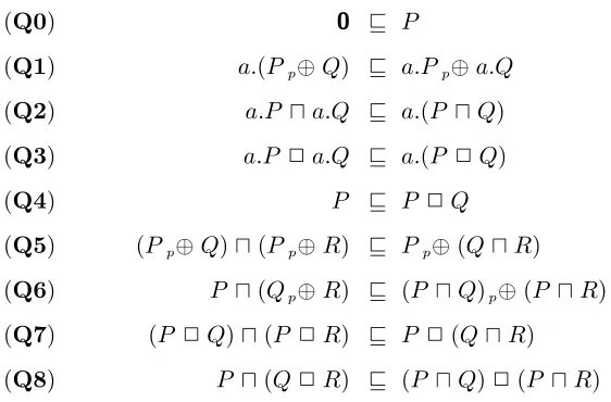
Because of the co-inductive nature of the definition of simulations we can begin to develop properties of the preorder ⊑S on pCSP terms. By Theorem 6.17, any equation P = Q or P ⊑ Q that we show to be sound for ≃S, respectively ⊑S, is also sound for ≃pmay, respectively ⊑pmay. In section 4 we have seen that many of the equations true for standard testing no longer apply to probabilistic processes. But some interesting identities can be salvaged.

Proposition 6.18 All the equations in Figure 8 are valid for≃S over pCSP.

Proof.

• _{Case (I1): It is clear that P ⊑S P ⊓ P since} [P ⊓ P℄ = P ⊓P

τ

−→ [P℄

and [P℄

S [P℄. For the inverse direction, observe that P ⊓ P

S [P℄ because

the transition P ⊓ P −→τ [P℄ is matched by [P℄

ˆ τ

=⇒ [P℄. Therefore we have [P ⊓P℄=P ⊓P

S [P℄, thus P ⊓P ⊑SP.

• _{Case (I3): Think for the moment of P ⊓Q⊓R as the ternary instance of a new}

auxiliary operatord_i∈IPi withI a finite index set, whose operational semantics consists of the transitionsd_i∈IPi −→τ Pifori∈I. Now we showP ⊓Q⊓R≃pmay (P ⊓Q)⊓R, and the proof ofP ⊓Q⊓R≃pmay P ⊓(Q⊓R) goes likewise.

ThatP ⊓Q⊓R

S (P ⊓Q)⊓Rfollows because a moveP ⊓Q⊓R τ

−→P can

be simulated by a sequence of two τ-steps from (P ⊓Q)⊓R. Conversely, that (P ⊓ Q) ⊓R

S P ⊓Q ⊓ R follows because the move (P ⊓Q)⊓R τ

−→ P ⊓ Q

can be simulated by the idle ˆτ-move P ⊓ Q ⊓ R −→τˆ P ⊓ Q ⊓ R and we have P ⊓ Q

S P ⊓ Q ⊓ R. The latter follows because any outgoing transition of P ⊓Qis also an outgoing transition of P ⊓Q⊓R.

(I1) P ⊓P =P

(I2) P ⊓Q =Q⊓P

(I3) (P ⊓Q)⊓R =P ⊓(Q⊓R)

(P1) Pp⊕P =P

(P2) Pp⊕Q =Q1−p⊕P

(P3) (Pp⊕Q)q⊕R =Pp·q⊕(Q(1−p)·q

1−p·q

⊕R)

(E1) P 20 _=P

(E2) P 2Q =Q2P

(E3) (P 2_Q)2R =P 2_(Q2_R)

(EI) a.P 2b.Q =a.P ⊓b.Q

(D1) P 2_{(Qp⊕R) = (P} 2_Q)p⊕(P 2_R)

(D2) a.P 2_{(Q⊓R) = (a.P} 2_Q)⊓(a.P 2_R)

(D3) P 2_{Q = (P1} 2_Q)⊓(P22_Q)⊓(P 2_Q1)⊓(P 2_Q2),

provided P =P1⊓P2, Q=Q1⊓Q2 (L1) P |AQ =Q|AP

(L2) 0_|A0 ₌0

(L3) 0_{|Aa.P =}  



a.(0_{|AP) ifa6∈A} 0 _ifa∈A

(L4) 0_{|A(P ⊓Q) = (}0_|AP)⊓(0_|AQ)

(L5) a.P |Ab.Q =

       

      

0 _{ifa, b∈Aand a6=b}

P |AQ ifa, b∈Aand a=b a.(P |Ab.Q) ifa6∈A and b∈A a.(P |Ab.Q)2b.(a.P |AQ) ifa, b6∈A

(L6) (P ⊓Q)|Aa.R =

 



(P |Aa.R)⊓(Q|Aa.R)⊓a.((P ⊓Q)|AR) ifa6∈A (P |Aa.R)⊓(Q|Aa.R) ifa∈A (L7) P |AQ = (P1 |AQ)⊓(P2 |AQ)⊓(P |AQ1)⊓(P |AQ2)

provided P =P1⊓P2, Q=Q1⊓Q2 (L8) P |A(Qp⊕R) = (P |AQ)p⊕(P |AR)