Detection Tool for Unbalanced Bids

http://www.scirp.org/journal/ojce ISSN Online: 2164-3172

ISSN Print: 2164-3164

DOI: 10.4236/ojce.2017.73028 Aug. 23, 2017 409 Open Journal of Civil Engineering

Detection Tool for Unbalanced Bids

Babak Nikpour1_{, Ahmed Senouci}2_{, Neil Eldin}2

1_{Field Project Controls, Arcadis, Chicago, USA}

2_{Department of Construction Management, University of Houston, Houston, USA}

Abstract

Unbalanced bidding is a cash flow management strategy that is recognized as an illegal/disqualifying practice by public owners; and unethical practice by most private owners. This practice provides the awarded bidder with unjusti-fied advantages at the expense of the owner. Unfortunately, limited tools and techniques are currently available to identify and detect unbalanced bids dur-ing the evaluation process. This paper presents an innovative detection tool to identify unbalanced bids in unit price contracts during the bid evaluation process. The proposed technique develops BMDI graphs to visualize total markup variation patterns during the project lifetime to detect unbalanced bids. The proposed method also uses Monte Carlo simulation to take in con-sideration the impact of cost uncertainties and risks. An illustrative example was presented to show the capabilities and features of the proposed method in determining the status of submitted bids during the evaluation process.

Keywords

Unbalanced Bidding, Detection, Bid Evaluation, Construction Projects, Monte-Carlo Simulation

1. Introduction

Cash flow management is a concern for contractors as payments from owners lag behind project expenditures. This time lag adversely affects the contractors’ cash flow and cause contractors to partially finance their projects. Unbalanced bidding, which is considered an illegal/unethical practice, may be used as a risky mitigation strategy [1]. Unbalanced bids can occur in fixed and unit price con-tracts. However, this study focuses on unbalanced bids in unit price concon-tracts. In unit price contracts, unbalanced bids can be prepared by manipulating the item’s prices without affecting the total bid price [2]. Unfortunately, it is usually diffi-How to cite this paper: Nikpour, B.,

Se-nouci, A. and Eldin, N. (2017) Detection Tool for Unbalanced Bids. Open Journal of Civil Engineering, 7, 409-422.

https://doi.org/10.4236/ojce.2017.73028

Received: July 21, 2017 Accepted: August 20, 2017 Published: August 23, 2017

Copyright © 2017 by authors and Scientific Research Publishing Inc. This work is licensed under the Creative Commons Attribution International License (CC BY 4.0).

DOI: 10.4236/ojce.2017.73028 410 Open Journal of Civil Engineering cult for owners to determine the existence and/or extent of potential infla-tion/deflation of bid item prices [2]. The difficulty comes from the fact that the award decision depends on the total bid price. The variations in the items’ unit prices are usually not considered. They may be due to legitimate reasons such as variations in the bidders’ expertise. They may also be due to a deliberate mani-pulation of unit prices to hide certain advantages, construction means, or pro-prietary technologies, or due to an honest mistake or a bad business decision.

Cattell [2] classifies unbalanced bids into three groups, namely, Front-End loaded, Back-End loaded, and Quantity Error Exploitation. Front-End loaded bids inflate the prices of early stage activities to positively impact the contractor cash-in flow. They usually result in owner overpayments when the value of time is considered [3]. In other words, Front-End bids allow for an interest-free loan from the owner to the contractor. Equally important, the overpayments would weaken the owner’s position and reduce the contractor’s incentives to complete the project. Back-End loading consists of inflating the prices of late schedule items. This pricing strategy is not common in relatively short duration construc-tion projects that located in low inflaconstruc-tion rate countries such as the United States. In Quantity Error Exploitation scenarios, the contractor increases the unit price of items in which actual quantities are expected to exceed the ones stated in the bid documents [2]. For example, in one of the contracts awarded by the Florida Department of Transportation (FDOT), the bid winner, inadvertent-ly or deliberateinadvertent-ly, offered a high unit price (i.e., $420/ft versus $171/ft) for trench support sheet. As the owner’s offered quantity was 30% of the actual one (i.e., 500 ft versus 1729 ft) the contractor was able to submit the lowest bid. Unfortu-nately, FDOT did not detect this problem, which resulted in additional unne-cessary cost of $516,180 [4]. Quantity Error Exploitation bids, which are more difficult to detect than other types, may have severe consequences on the owner cost.

The US public and private sectors have different approaches to unbalanced bids. The federal code of regulation (48 C.F.R. § 15.404−1 (g)) forbids unba-lanced pricing because of its adverse consequences on performance risk and payments. However, unbalanced bids are not forbidden in the US private con-struction industry sector. However, they are considered as unethical and risky acts. Moreover, the private sector strives to detect unbalanced bids in advance as a preventive action.

DOI: 10.4236/ojce.2017.73028 411 Open Journal of Civil Engineering

2. Literature Review

A literature review was conducted to determine the state-of-the-art in the area of unbalanced bids. In 2004, the American Association of State Highway and Transportation Officials (AASHTO) conducted a survey about how State De-partment of Transportation (DOT) agencies were handling unbalanced bids [8]. A total of 27 State DOTs responded to the survey. The survey results showed that most states did not have any formal procedure to detect unbalanced bids. Florida DOT used a statistical analysis approach to define an acceptable range for each line item price. It also developed a computer program that automatical-ly detects any out of range item price. Texas DOT defined an acceptable range for each line item based on engineering estimates. Then, the possible monthly payments trends of the first and second bidders were computed using the pro-posed bidders’ time schedules. The two trends were then compared to help the evaluators find out unbalanced bids. North Carolina DOT used a contractual provision to prevent unreasonable line item prices. Unit or lump sum prices were considered reasonable and acceptable if they were close to the average of the engineering estimate and other bidder prices. Wang [9] developed a bid-der-based quantitative approach that examined separately every line item price using four tasks, namely, preparation, evaluation, explanation, and adjustment. Arditi and Chotibhongs [10] developed two automated Excel spreadsheet pro- cessing models to detect mathematically and materially unbalanced bids. The models compare the price of each line item against engineering estimates and other bidders’ prices. Shrestha and Joshi [11] conducted a statistical analysis on a historical data set that was collected from 264 bids for 70 road projects to inves-tigate if the submitted bids were unbalanced. Skitmore and Cattell [12] used si-mulation to investigate the impact of two common errors commonly made by bid evaluators. Hyari [13] developed a bid rebalancing model that is based on prevention of unbalanced bids rather than their detection. The model adjusts all line item prices of the lowest bids.

Simulation Methods

DOI: 10.4236/ojce.2017.73028 412 Open Journal of Civil Engineering

3. Method Formulation

3.1. Bid Markup Distribution Index Graphs

The total bid price is computed by adding expected profits to estimated con-struction and overhead costs. Project concon-struction cost can be determined fairly accurately using project documents, such as drawings and specifications. How-ever, overhead costs and profit are more difficult to estimate accurately and can be affected by many factors, such as market conditions, or bidders’ need for the job [16]. The amount of general overhead cost and profit is often specified as a markup amount or a percentage of total bid price, for example, 15% of total construction cost [16]. The markup amount is then distributed among project construction activities. The distribution of the overall markup amount in each activity can affect cash-flow of the bidder [17]. For example, by inflating the markup amount for early activities and deflating it for late activities, bidders can improve their cash-flow and reduce their interest costs [16]. Furthermore, the bidder’s profit can be increased by manipulating the markup distribution in case of expected errors in the quantity of work provided by the owner’s representa-tive.

The markup distribution in fixed and unit price contracts’ biddings is differ-ent from each other. However, the basic idea of distributing the overall markup to activities is similar. One of the methods to distribute the overall markup is to allocate the markup amounts proportionally to the cost of each activity. Mincks and Johnston [17] used the activity cost to total cost ratios to compute the activ-ity markup amounts. This is a simple method that leads to a “balanced” activactiv-ity markup. However, a “balanced” markup distribution does not likely leads to an improved cash flow. That’s why, bidders frequently use “unbalanced” markup distributions methods to improve their project cash flows.

DOI: 10.4236/ojce.2017.73028 413 Open Journal of Civil Engineering Figure 1. BMDI graph for front-end loaded bids.

Figure 2. BMDI graph for back-end loaded bids.

DOI: 10.4236/ojce.2017.73028 414 Open Journal of Civil Engineering Figure 4. BMDI graph for balanced bids.

for balanced bids, which shows a relatively constant markup distribution along the project life time.

3.2. Proposed Method Development

The proposed method develops bid BMDI graphs to visualize total markup vari-ation patterns during the project lifetime and to detect unbalanced bids. It also uses Monte Carlo simulation to take in consideration the impact of cost uncer-tainties and risks. Monte Carlo simulation uses random generated numbers to evaluate the impact of uncertain factors on the final results. Triangular probabil-ity distributions were used herein to simulate possible bid item unit costs and quantities. The upper, lower, and most likely values can be estimated using in-ternal company records, commercially published books, or expert judgements. The proposed method consists of the following three major computational steps:

3.2.1. Input Data

For each bid item, all unit prices are read and compiled. A pseudo code of the computational tasks in this step is shown below.

For each bid item i (i = 1, ∙∙∙, I), where I = number of bid items. For each bidder m (m = 1, ∙∙∙, M), where M = number of bidders. • _{Read bid item unit price-BIUP (i, m).}

• _{Read bid item quantity-BIEQ (i).}

3.2.2. Monte-Carlo Simulation

Triangular probability distributions were used herein for BIEQs and BIEUCs. Moreover, the number of simulation iterations was set equal to 5000. The Monte-Carlo simulation is described using the following pseudo code:

DOI: 10.4236/ojce.2017.73028 415 Open Journal of Civil Engineering

( )

( )

m BIUP i m

M BIEUC i =         = +

∑

where % Markup = percent cost markup (typically equal to 15%) and M = number of bids.

• _{Calculate bid item price BIEC (i) using the following equation:}

( )

( )

( )

BIEC i =BIEQ i ∗BIEUC i (2)

• _{Estimate the minimum, maximum, and most likely values of bid item} quan-tity, BIEQ (i).

• _{Estimate the minimum, maximum, and most likely values of bid item unit} cost, BIEUC (i).

For each simulation iteration r (r = 1, ∙∙∙, R), where R = total number of itera-tions.

For each bid item i (i = 1, ∙∙∙, I), where I = number of bid items. • _{Generate random values for BIEQ (r, i) and BIEUC (r, i).}

• _{For each bidder and for each monitoring period (t = 1, ∙∙∙, T), where T = total} number of monitoring periods.

o Compute BMDI (r, m, t) using the following equation:

(

)

(

)

( )

(

)

( )

( )

(

)

BIEP r i m

Act i m t Dur i m

BMDI r m t

BIEC r i

Act i m t Dur i m

= = ∗ = ∗

∑

∑

where: BMDI (r, m, t) = bid markup distribution index in iteration r for bidder m during monitoring period t; Dur (i, m) = scheduled duration of bid item i, of-fered by bidder m; Act (i, m, t) = number of active periods of bid item i, counted in the offered time schedule by bidder m, for monitoring period t.

3.2.3. BMDI Graphs

All generated BMDI values will be used herein to generate five separate tend lines, namely, minimum, 1st quarter, median, 3rd quarter, and maximum. The bid balance status (i.e., balanced or unbalanced) and potential risks will be de-termined by interpreting the patterns of these trend lines.

The computational tasks for the generation of the BMDI trend lines are sum-marized using the following pseudo code:

For each bidder m (m = 1, ∙∙∙, M), where M = total number of bidders.

For each monitoring period t (t = 1, ∙∙∙, T), where T = total number of moni-toring periods.

• _{Determine the minimum, 1st quarter, median, 3rd quarter, and maximum} BMDI values.

DOI: 10.4236/ojce.2017.73028 416 Open Journal of Civil Engineering • _{Analyze the bidders BMDI graphs to determine the status of the submitted}

bids.

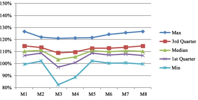
4. Illustrative Example

An illustrative example is used herein to show the capabilities and features of the proposed method. It consists of a 13-activity construction project and is 30 weeks long. BMDI values will be calculated and monitored for 8 months. Figure 5 shows the Gantt chart project schedule.

4.1. Balanced Bids

In a balanced bid, the project total markup is distributed evenly among project activities. Table 1 summarizes the computation of the BMDI values in the case of a balanced bid.

Figure 5. Gantt chart project schedule.

Table 1. Balanced loaded bid scenario.

Bid items BIUP BIEUC Markup BIEQ BIEUC

Min Most likely Max Min Most likely Max A 4.57 $/m 4.00 $/m 114% 68,835 m 72,765 m 83,160 m 3.60 $/m 4.20 $/m 4.60 $/m B 12.78 $/m 11.20 $/m 114% 27,930 m 30,870 m 35,280 m 10.08 $/m 11.76 $/m 12.88 $/m C 5.83 $/m 5.00 $/m 117% 33,250 m 36,750 m 42,000 m 4.50 $/m 5.25 $/m 5.75 $/m D 5.20 $/m 4.55 $/m 114% 27,930 m 30,870 m 35,280 m 4.10 $/m 4.78 $/m 5.23 $/m E 11.53 $/m 10.00 $/m 115% 25,935 m 28,665 m 32,760 m 9.00 $/m 10.50 $/m 11.50 $/m F 5.48 $/m 4.80 $/m 114% 53,200 m 58,800 m 67,200 m 4.32 $/m 5.04 $/m 5.52 $/m G 7.40 $/m 6.20 $/m 119% 53,865 m 59,535 m 68,040 m 5.58 $/m 6.51 $/m 7.13 $/m H 6.03 $/m 5.30 $/m 114% 33,250 m 36,750 m 42,000 m 4.77 $/m 5.57 $/m 6.10 $/m I 11.90 $/m 10.50 $/m 113% 21,280 m 23,520 m 26,880 m 9.45 $/m 11.03 $/m 12.08 $/m J 9.72 $/m 8.50 $/m 114% 29,260 m 32,340 m 36,960 m 7.65 $/m 8.93 $/m 9.78 $/m K 4.04 $/m 3.50 $/m 115% 51,870 m 57,330 m 65,520 m 3.15 $/m 3.68 $/m 4.03 $/m L 7.21 $/m 6.30 $/m 114% 53,200 m 58,800 m 67,200 m 5.67 $/m 6.62 $/m 7.25 $/m M 57.40 $/m 50.20 $/m 114% 5320 m 5880 m 6720 m 45.18 $/m 52.71 $/m 57.73 $/m

DOI: 10.4236/ojce.2017.73028 417 Open Journal of Civil Engineering Figure 6 shows that the 5 BMDI trend lines are almost horizontally during the project time. Moreover, the minimum maximum and middle trend lines follow the same direction.

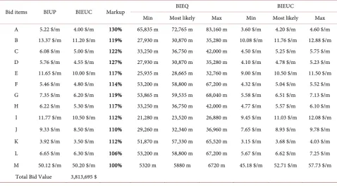
4.2. Front-End Loaded Bids

In front-end loaded bids, early stage activities have bigger markups than late stage activities. Table 2 summarizes the computation of BMDI values in a front- end loaded bid scenario. Figure 7 shows a decreasing pattern for the 5 BMDI trend lines. Moreover, the minimum maximum and middle trend lines follow the same direction.

Figure 6. BMDI values variation with project time in a balanced bid.

Table 2. Front-End loaded bid scenario.

Bid items BIUP BIEUC Markup BIEQ BIEUC

Min Most likely Max Min Most likely Max A 5.22 $/m 4.00 $/m 130% 65,835 m 72,765 m 83,160 m 3.60 $/m 4.20 $/m 4.60 $/m B 13.37 $/m 11.20 $/m 119% 27,930 m 30,870 m 35,280 m 10.08 $/m 11.76 $/m 12.88 $/m C 6.08 $/m 5.00 $/m 122% 33,250 m 36,750 m 42,000 m 4.50 $/m 5.25 $/m 5.75 $/m D 5.76 $/m 4.55 $/m 127% 27,930 m 30,870 m 35,280 m 4.10 $/m 4.78 $/m 5.23 $/m E 11.65 $/m 10.00 $/m 117% 25,935 m 28,665 m 32,760 m 9.00 $/m 10.50 $/m 11.50 $/m F 5.46 $/m 4.80 $/m 114% 53,200 m 58,800 m 67,200 m 4.32 $/m 5.04 $/m 5.52 $/m G 7.35 $/m 6.20 $/m 119% 53,865 m 59,535 m 68,040 m 5.58 $/m 6.51 $/m 7.13 $/m H 6.22 $/m 5.30 $/m 117% 33,250 m 36,750 m 42,000 m 4.77 $/m 5.57 $/m 6.10 $/m I 11.77 $/m 10.50 $/m 112% 21,280 m 23,520 m 26,880 m 9.45 $/m 11.03 $/m 12.08 $/m J 9.33 $/m 8.50 $/m 110% 29,260 m 32,340 m 36,960 m 7.65 $/m 8.93 $/m 9.78 $/m K 3.92 $/m 3.50 $/m 112% 51,870 m 57,330 m 65,520 m 3.15 $/m 3.68 $/m 4.03 $/m L 6.65 $/m 6.30 $/m 106% 53,200 m 58,800 m 67,200 m 5.67 $/m 6.62 $/m 7.25 $/m M 50.12 $/m 50.20 $/m 100% 5320 m 5880 m 6720 m 45.18 $/m 52.71 $/m 57.73 $/m

DOI: 10.4236/ojce.2017.73028 418 Open Journal of Civil Engineering Figure 7. BMDI values variation with project time in a fron-end loaded bid.

4.3. Back-End Loaded Bids

In back-end loaded bids, late stage activities have bigger markups than early stage activities. Table 3 summarizes the computation of the BMDI values in a back-end loaded bid scenario Figure 8 shows an increasing pattern for the 5 BMDI trend lines. Moreover, the minimum maximum and middle trend lines follow the same direction.

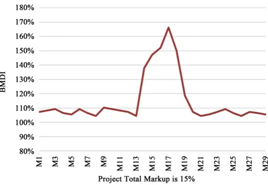
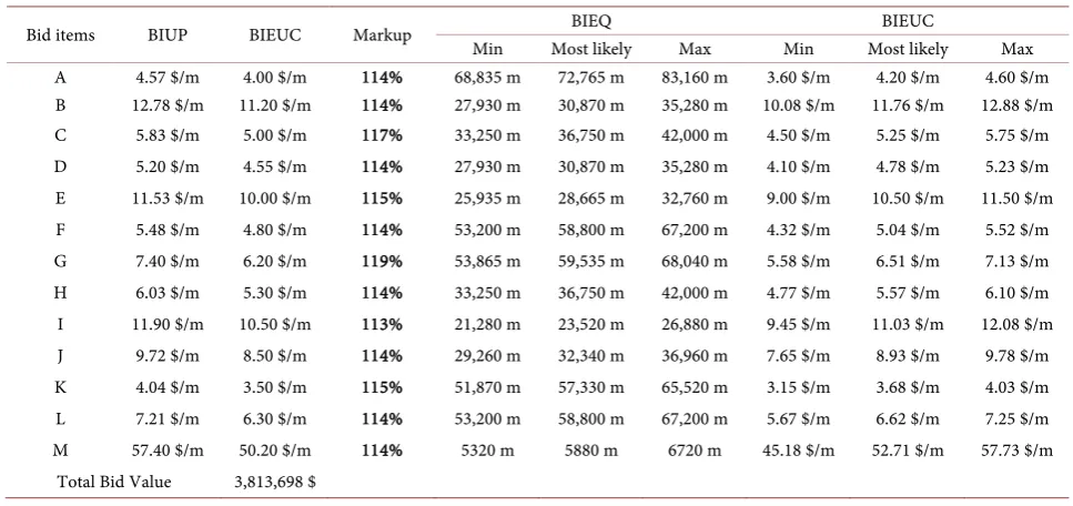
4.4. Quantity Error Exploitation Unbalanced Bids

The bidder believes herein that the owner has underestimated the quantity amount of a bid item such as item E. To take advantage of this oversight, the bidder increased the unit price of item E and decreased the unit price of the oth-er items expecting a biggoth-er markup value for item E than for othoth-er items. Table 4 the computation of the BMDI values in the case of a back-end loaded bid. Figure 9 shows a spike in the 5 BMDI trend lines in the middle of the project when item E is active. This pattern is typical for Quantity Error Exploitation unbalanced bids.

4.5. Risk Analysis

There is always a risk that item unit costs vary in an uncontrolled manner. This affects not only the markup of that bid item but also the project markup. For example, let us consider that there is a risk that the expected cost of activity G increases from $7.13/m to $11.16/m (Table 5). This risk is reflected by a drop in minimum BMDI trend line as shown in Figure 10. This kind of pick/drop can be a sign of a risk in a BMDI graph.

5. Conclusion

DOI: 10.4236/ojce.2017.73028 419 Open Journal of Civil Engineering Figure 8. BMDI values variation with project time in a back-end loaded bid.

Figure 9. BMDI values variationwith project time for quantity error exploitation bids.

Table 3. Back-end loaded bid scenario.

Bid items BIUP BIEUC Markup BIEQ BIEUC

DOI: 10.4236/ojce.2017.73028 420 Open Journal of Civil Engineering Table 4. Quantity error exploitation bid scenario.

Bid items BIUP BIEUC Markup BIEQ BIEUC

Min Most likely Max Min Most likely Max

A 4.12 $/m 4.00 $/m 103% 65,835 m 72,765 m 83,160 m 3.60 $/m 4.20 $/m 4.60 $/m

B 11.52 $/m 11.20 $/m 103% 27,930 m 30,870 m 35,280 m 10.08 $/m 11.76 $/m 12.88 $/m

C 5.15 $/m 5.00 $/m 103% 33,250 m 36,750 m 42,000 m 4.50 $/m 5.25 $/m 5.75 $/m

D 4.68 $/m 4.55 $/m 103% 27,930 m 30,870 m 35,280 m 4.10 $/m 4.78 $/m 5.23 $/m

E 25.00 $/m 10.00 $/m 250% 25,935 m 28,665 m 32,760 m 9.00 $/m 10.50 $/m 11.50 $/m

F 4.94 $/m 4.80 $/m 103% 53,200 m 58,800 m 67,200 m 4.32 $/m 5.04 $/m 5.52 $/m

G 6.38 $/m 6.20 $/m 103% 53,865 m 59,535 m 68,040 m 5.58 $/m 6.51 $/m 7.13 $/m

H 5.45 $/m 5.30 $/m 103% 33,250 m 36,750 m 42,000 m 4.77 $/m 5.57 $/m 6.10 $/m

I 10.80 $/m 10.50 $/m 103% 21,280 m 23,520 m 26,880 m 9.45 $/m 11.03 $/m 12.08 $/m

J 8.75 $/m 8.50 $/m 103% 29,260 m 32,340 m 36,960 m 7.65 $/m 8.93 $/m 9.78 $/m

K 3.60 $/m 3.50 $/m 103% 51,870 m 57,330 m 65,520 m 3.15 $/m 3.68 $/m 4.03 $/m

L 6.48 $/m 6.30 $/m 103% 53,200 m 58,800 m 67,200 m 5.67 $/m 6.62 $/m 7.25 $/m

M 51.66 $/m 50.20 $/m 103% 5320 m 5880 m 6720 m 45.18 $/m 52.71 $/m 57.73 $/m

Total Bid Value 3,813,697 $

Table 5. Risk analysis scenario.

Bid items BIUP BIEUC Markup BIEQ BIEUC

Min Most likely Max Min Most likely Max

A 4.57 $/m 4.00 $/m 114% 65,835 m 72,765 m 83,160 m 3.60 $/m 4.20 $/m 4.60 $/m

B 12.78 $/m 11.20 $/m 114% 27,930 m 30,870 m 35,280 m 10.08 $/m 11.76 $/m 12.88 $/m

C 5.83 $/m 5.00 $/m 117% 33,250 m 36,750 m 42,000 m 4.50 $/m 5.25 $/m 5.75 $/m

D 5.20 $/m 4.55 $/m 114% 27,930 m 30,870 m 35,280 m 4.10 $/m 4.78 $/m 5.23 $/m

E 11.53 $/m 10.00 $/m 115% 25,935 m 28,665 m 32,760 m 9.00 $/m 10.50 $/m 11.50 $/m

F 5.48 $/m 4.80 $/m 114% 53,200 m 58,800 m 67,200 m 4.32 $/m 5.04 $/m 5.52 $/m

G 7.40 $/m 6.20 $/m 119% 53,865 m 59,535 m 68,040 m 5.58 $/m 6.51 $/m 13.64 $/m

H 6.03 $/m 5.30 $/m 114% 33,250 m 36,750 m 42,000 m 4.77 $/m 5.57 $/m 6.10 $/m

I 11.90 $/m 10.50 $/m 113% 21,280 m 23,520 m 26,880 m 9.45 $/m 11.03 $/m 12.08 $/m

J 9.72 $/m 8.50 $/m 114% 29,260 m 32,340 m 36,960 m 7.65 $/m 8.93 $/m 9.78 $/m

K 4.04 $/m 3.50 $/m 115% 51,870 m 57,330 m 65,520 m 3.15 $/m 3.68 $/m 4.03 $/m

L 7.21 $/m 6.30 $/m 114% 53,200 m 58,800 m 67,200 m 5.67 $/m 6.62 $/m 7.25 $/m

M 57.40 $/m 50.20 $/m 114% 5320 m 5880 m 6720 m 45.18 $/m 52.71 $/m 57.73 $/m

DOI: 10.4236/ojce.2017.73028 421 Open Journal of Civil Engineering Figure 10. BMDI graph risk visualization.

most of unbalanced bidders lose their financial motivation during the project. Unfortunately, the bid evaluation process is usually conducted under time pres-sure. Moreover, the evaluators usually use unreliable and time consuming qua-litative approaches to detect unbalanced bids. BMDI graphs are as an innovative visual detection tool that helps owners analyze and compare submitted bids and support their awarding process quickly and reliably. The tool visualizes project markup variation patterns during its lifetime to detect unbalanced bids. It also uses Monte Carlo simulation to take in consideration the impact of cost uncer-tainties and risks.

References

[1] Cui, Q.B., Hastak, M. and Halpin, D. (2010) Systems Analysis of Project Cash Flow Management Strategies. Construction Management and Economics, 28, 361-376.

https://doi.org/10.1080/01446191003702484

[2] Cattell, D., Bowen, P. and Kaka, A. (2007) Review of Unbalanced Bidding Models in Construction. Journal of Construction Engineering & Management, 133, 562-573.

https://doi.org/10.1061/(ASCE)0733-9364(2007)133:8(562)

[3] McGreevy, S.L. (2002) Unbalanced Bids Are Risky Business.

http://www.contractormag.com/articles/column.cfm?columnid=161

[4] Hyari, K., Tarawneh, Z. and Katkhuda, H. (2016) Detection Model for Unbalanced Pricing in Construction Projects: A Risk-Based Approach. Journal of Construction Engineering & Management, 142, 1-10.

https://doi.org/10.1061/(ASCE)CO.1943-7862.0001203

[5] Hoogenboom, J., Dale, W. and Martell, C. (2006) Risk Analysis and Optimization of the (Un)balanced Bid. AACE International transactions, 7, 1-6.

[6] Cattell, D., Bowen, P. and Kaka, A. (2008) A Simplified Unbalanced Bidding Model.

Construction Management and Economics, 26, 1283-1290.

https://doi.org/10.1080/01446190802570506

[7] Liu, X., Lin, L. and Zang, D. (2009) Stochastic Programming Models and Hybrid Intelligent Algorithm for Unbalanced Bidding Problem. Journal of Computing and Information Science in Engineering, 2, 188-194.

https://doi.org/10.5539/cis.v2n1p188

DOI: 10.4236/ojce.2017.73028 422 Open Journal of Civil Engineering DOT Procedures for the Evaluation of Materially Unbalanced Bids. American As-sociation of State Highway and Transportation Officials, Washington DC.

[9] Wang, W. (2004) Electronic-Based Procedure for Managing Unbalanced Bids.

Journal of Construction Engineering & Management, 130, 455-460.

https://doi.org/10.1061/(ASCE)0733-9364(2004)130:3(455)

[10] Arditi, D. and Chotibhongs, R. (2009) Detection and Prevention of Unbalanced Bids. Construction Management and Economics, 27, 721-732.

https://doi.org/10.1080/01446190903117785

[11] Shrestha, P.P., Shrestha, K. and Joshi, V. (2012) Investigation of Unbalanced Bid-ding for Economic Sustainability. Proceedings of International Conference on Sus-tainable Design, Engineering, and Construction, Fort Worth, 7-9 November 2012, 609-615.

[12] Skitmore, M. and Cattell, D. (2013) On Being Balanced in an Unbalanced World.

Journal of the Operational Research Society, 64, 138.

https://doi.org/10.1057/jors.2012.29

[13] Hyari, K.H. (2015) Handling Unbalanced Bidding in Construction Projects: Preven-tion Rather than DetecPreven-tion. Journal of Construction Engineering & Management, 142, 1-10. https://doi.org/10.1061/(ASCE)CO.1943-7862.0001045

[14] Afshar, A. and Amiri, H. (2010a) A Min-Max Regret Approach to Unbalanced Bid-ding in Construction. KSCE Journal of Civil Engineering, 14, 653-661.

https://doi.org/10.1007/s12205-010-0972-0

[15] Afshar, A. and Amiri, H. (2010b) Risk-Based Approach to Unbalanced Bidding in Construction Projects. Optim Engineering, 42, 369-385.

https://doi.org/10.1080/03052150903220964

[16] Peterson, S.J. (2009) Construction Accounting and Financial Management. Pearson Education, Inc., Upper Saddle River.

[17] Mincks, W.R. and Johnston, H. (2011) Construction Jobsite Management. 3rd Edi-tion, Delmar Cengage Learning, Clifton Park.

[18] Shim, E. and Kim, S.J. (2016) Cost Item-Based Markup Distribution in Construc-tion Projects. The Journal of Technology, Management, and Applied Engineering, 32, 1-26.

Submit or recommend next manuscript to SCIRP and we will provide best service for you:

Accepting pre-submission inquiries through Email, Facebook, LinkedIn, Twitter, etc. A wide selection of journals (inclusive of 9 subjects, more than 200 journals)

Providing 24-hour high-quality service User-friendly online submission system Fair and swift peer-review system

Efficient typesetting and proofreading procedure

Display of the result of downloads and visits, as well as the number of cited articles Maximum dissemination of your research work

Submit your manuscript at: http://papersubmission.scirp.org/