Polarizations as States and Their Evolution in Geometric Algebra Terms with Variable Complex Plane

(1)

http://www.scirp.org/journal/jamp ISSN Online: 2327-4379

ISSN Print: 2327-4352

DOI: 10.4236/jamp.2018.64063 Apr. 20, 2018 704 Journal of Applied Mathematics and Physics

Polarizations as States and Their Evolution in

Geometric Algebra Terms with Variable

Complex Plane

Alexander Soiguine

SOiGUINE Quantum Computing, Aliso Viejo, CA, USA

Abstract

Recently suggested scheme [1] of quantum computing uses g-qubit states as circular polarizations from the solution of Maxwell equations in terms of geometric algebra, along with clear definition of a complex plane as bivector in three dimensions. Here all the details of receiving the solution, and its pola-rization transformations are analyzed. The results can particularly be applied to the problems of quantum computing and quantum cryptography. The sug-gested formalism replaces conventional quantum mechanics states as objects constructed in complex vector Hilbert space framework by geometrically feasible framework of multivectors.

Keywords

Quantum Mechanics, Quantum Computing, Geometric Algebra, Maxwell Equations

1. Introduction

The circular polarized electromagnetic waves are the only type of waves follow-ing from the solution of Maxwell equations in free space done in geometric al-gebra terms.

Let’s take the electromagnetic field in the form:

(

)

0exp S

F=F _I ωt− ⋅k r _ (1)

requiring that it satisfies the Maxwell system of equations in free space, which in geometrical algebra terms is one equation:

(

∂ + ∇t

)

F =0 (2) How to cite this paper: Soiguine, A. (2018)

Polarizations as States and Their Evolution in Geometric Algebra Terms with Variable Complex Plane. Journal of Applied Ma-thematics and Physics, 6, 704-714. https://doi.org/10.4236/jamp.2018.64063

Received: March 7, 2018 Accepted: April 17, 2018 Published: April 20, 2018

http://creativecommons.org/licenses/by/4.0/

(2)

DOI: 10.4236/***.2018.***** 705 Journal of Applied Mathematics and Physics

where ˆ ˆ ˆ

xx yy zz

∂ ∂ ∂

∇ = + +

∂ ∂ ∂ and multiplications are the geometrical algebra

ones.

Element F0 in (1) is a constant element of geometric algebra G3 and IS is unit value bivector of a plane S in three dimensions, that is a generalization of the imaginary unit [2], [3]. The exponent in (1) is unit value element of G3

+ _[3]: eIS cos sin ,

S

I t

ϕ ₌

_ϕ

₊

_{ϕ ϕ ω}

₌ _{− ⋅} k r

Solution of (2) should be sum of a vector (electric field E) and bivector (mag-netic field I H3 ):

3

F= +E I H with some initial conditions:

3 t0, 0 0 t0, 0 3 t0, 0 0 3 0

I ₌ ₌ F ₌ ₌ I ₌ ₌ I

+ _r = = _r + _r = +

E H E H E H

In the magnetic field I H3 the item I3 is unit pseudoscalar in three

dimen-sions assumed to be the right-hand screw oriented volume, relative to an or-dered triple of orthonormal vectors.

Substitution of (1) into the Maxwell’s (2) will exactly show us what the solu-tion looks like.

2. Solution in the Geometric Algebra Terms

The derivative by time gives

(

)

0e 0e

S S

I I

S S S

F F I t F I FI

t t

ϕ _ω ϕ _ω _ω

∂ ₌ ∂ _{− ⋅ =} ₌

∂ ∂ k r

The geometric algebra product ∇F is:

(

)

0 e 0e

S S

I I

S S S

F F I ϕ ωt F ϕI FI

∇ = ∇ − ⋅k r = − k= − k

or

(

)

0e 0e

S S

I I

S S S

F F ϕ ωt I F ϕ I F I

∇ = ∇ − ⋅k r = − k = − k ,

depending on do we write IS

(

ω

t− ⋅k r

)

or

(

ω

t− ⋅k r

)

IS. The result should be the same since ωt− ⋅k r is a scalar.

Commutativity ISk=kIS is true only if k×I I3 S =0. The following agree-ment takes place between orientation of I3, orientation of IS and direction of vector k [3]. The vector I I3 S =I IS 3 is orthogonal to the plane of IS and its direction is defined by orientations of I3 and IS. Rotation of right/left hand screw defined by orientation of IS gives movement of right/left hand screw. This is the direction of the vector I I3 S =I IS 3. That means that the matching

between

_k

ˆ

_and S

I should be kˆ= ±I I3 S or kIˆS =I3 1_.

Assuming that orientation is I3=kIˆS, the Maxwell equation becomes:

(

S I3

)

(

S kˆS

)

0

F I ω− k =F ωI − k I =

or

(3)

(

E+I3H

)

ω

=

(

E+I3H k

)

Left hand side is sum of vector and bivector, while right hand side is scalar ⋅

E k plus bivector E∧k , plus pseudoscalar I3

(

H k⋅

)

, plus vector

(

)

3

I H∧k . It follows that both E and H lie on the plane of IS and then: 2

3 , 3 2 3

I I ω I

ωE= Hk ω H=Ek→ Hk=ωE

k

Thus,

ω

= k and we get equation I3Hkˆ=E from which particularly fol-lows 2 2

=

E H and _EkHˆ ˆˆ ₌_I₃.

The result for the case I3=kIˆS is that the solution of (2) is

(

0 3 0

)

exp S

(

)

F= E +I H _I ωt− ⋅k r _

where E0 and H0 are arbitrary mutually orthogonal vectors of equal length,

lying on the plane S. Vector k should be normal to that plane, kˆ= −I I3 S and

ω

=

k .

In the above result the sense of the IS orientation and the direction of 𝑘𝑘�⃗ were assumed to agree with I3=kIˆS. Opposite orientation, − =I3 kIˆS, that’s k

and IS compose left hand screw and kˆ=I I3 S , will give solution

(

)

0exp S

F=F _I ωt− ⋅k r _ with _EHkˆ ˆˆ₌_I₃. Summary:

For a plane S in three dimensions Maxwell equation (2) has two solutions • F₊=

(

E₀+I₃H₀

)

exp_I_S

(

ωt−k₊⋅r

)

_, with kˆ+ =I I₃ _S,EHkˆ ˆˆ+=I3, and the

triple

{

_{E H k}ˆ ˆ_, _,ˆ

}

+ is right hand screw oriented, that’s rotation of Eˆ to Hˆ by π/2 gives movement of right hand screw in the direction of k+= k I I3 S.

• F₋=

(

E₀+I₃H₀

)

exp_I_S

(

ωt−k₋⋅r

)

_, with kˆ−= −I I₃ _S,EHkˆ ˆˆ−= −I3, and the triple

{

_{E H k}ˆ ˆ_, _,ˆ

}

− is left hand screw oriented, that’s rotation of Eˆ to Hˆ by π/2 gives movement of left hand screw in the direction of k−= −k I I3 S or, equivalently, movement of right hand screw in the opposite direction,

−

−k .

• _E₀ _and_H₀_{, initial values of}_E_and_H_{, are arbitrary mutually orthogonal} vec-tors of equal length, lying on the plane S. Vectors k±= ±k± I I3 S are normal to that plane. The length of the wave vectors k± is equal to angular fre-quency ω_.

Maxwell Equation (2) is a linear one. Then any linear combination of F+ and F− saving the structure of (1) will also be a solution.

Let’s write:

(

)

[

]

(

)

(

)

[

]

(

)

0 3 0 3

exp exp exp exp

S S S

F I I t I I I

ω

+

−

 = + − _ ⋅ _

  



  

= + ⋅

 _ _ __



E H r

E H r (3)

Then for arbitrary scalars λ and μ:

(

)

(

(3 ) (3 )

)

0 3 0 e e e

S S S S

S I I I I I I

I t

F F I ω

λ µ λ − _ ⋅_ µ _ ⋅_

++ −= + +

r r

E H (4)

(4)

DOI: 10.4236/***.2018.***** 707 Journal of Applied Mathematics and Physics of two states with the same phase in the same plane but opposite sense of orien-tation. The states are strictly coupled, entangled if you prefer, because bivector plane should be the same for both, does not matter what happens with it.

One another option is:

(

)(

)

(

)

(

)(

)

(

)

(

)

(

)

(

)

(

)

1 3 1 0 3 0 3

2 3 2 0 3 0 3

1 0 1 0 3 1 0 1 0 3

2 0 2 0 3 2 0 2 0 3

exp exp

S S

I I I t I I

I I t I I

λ µ ω

λ µ µ λ ω

 

+ + _ − ⋅ _

 

+ + + _ + ⋅ _

 

=_ − + + _ _ − ⋅ _

 

+_ − + + _ _ + ⋅ _

E H r

E H E H r

which is just rotation, along with possible change of length, of electric and mag-netic initial vectors in their plane.

3. Transformations of Polarization States

Polarizations, in our approach, exponents in the solution of (3), have the form of states [3], that’s elements of G3

+_:

3 cos sin eS

I

S S

G+

α

+I

β

≡

ϕ

+I

ϕ

= ϕ, distri-buted in

( )

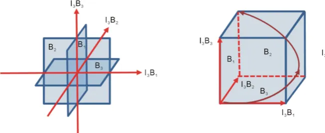
t r, space. They are operators than can act on observables, also ele-ments of G3, particularly other polarizations. Such states can be depicted in the

current geometric algebra formalism using a triple of basis bivectors in three dimensions

{

B B B1, 2, 3

}

(Figure 1):

The basis bivectors satisfy multiplication rules (in the righth and screw orien-tation of I3):

1 2 3

B B = −B , B B1 3=B2, B B2 3= −B1

One can identify basis bivectors with usual coordinate planes: B1=yzˆ ˆ,

2 ˆˆ

B =zx, B3=xyˆˆ. Any one of these three bivectors can be taken as explicitly

identifying imaginary unit, though any unit value bivector in three dimensions can take the role [2], [4].

Thus:

(

1 1 2 2 3 3

)

1 1 2 2 3 3

S

I b B b B b B B B B

α

+

β α β

= + + + ≡ +

α β

+

β

+

β

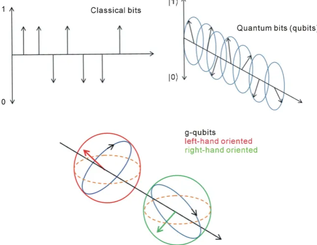
[image:4.595.209.535.567.701.2]

The difference between units of information in classical computational scheme, quantum mechanical conventional computations (qubits) and geometric algebra

(5)

[image:5.595.212.535.453.702.2]

DOI: 10.4236/***.2018.***** 708 Journal of Applied Mathematics and Physics scheme (g-qubits) with variable explicitly defined complex plane is seen from Figure 2.

Circular polarizations received as solutions of Maxwell Equation (2) is an ex-cellent choice to have such g-qubits in a lab.

Commonly accepted idea to use systems of qubits to tremendously increase speed of computations is based on assumption of entanglement – roughly speaking when touching one qubit all the other in the system react instantly, in no time. A bit strange, though you should not care about that because our para-digm is very different.

Assume we have some general state:

(

1 1 2 2 3 3

)

1 1 2 2 3 3

S

I b B b B b B B B B

α

+

β α β

= + + + ≡ +

α β

+

β

+

β

The state can be identified as a point

(

α β β β

1, 1, 2, 3

)

on unit sphere 3

S . It can be subjected to a Clifford translation

(

)

eICl

S S

I ψ I

α₊ β _⇒ ∆ α₊ β

executing displacement ∆ψ at point

(

α β β β

1, 1, 2, 3

)

along intersection of 3

S with the unit bivector plane ICl.

Let’s make notations more like conventional quantum mechanical ones. I will write:

( , ,S), ( , ,S)

S I S S I

I g _{α β} I I g _{α β}

α+ β≡ α+ β α= − β ≡

and use Hamiltonian like form of the Clifford translation bivector. Conventional Hamiltonian

(6)

1 2 3

2 3 1

i i

γ γ γ γ

+ −

 

 ₊ ₋ 

 ,

with removed not important scalar γ, has the lift in G3

+ _[3]:

(

)

3 1 1 2 2 3 3

I

γ

B

γ

B

γ

B

= + +



Then the associated Clifford translation plane bivector is −I3

( )

t . By

nor-malizing the bivector to unit value we get generalization of imaginary unit

( )

3

t

i I

t

⇒ 

 ,

that is critical for the whole approach. Therefore, for some Δt, Clifford transla-tion for a given Hamiltonian is:

(

)

₍ ₍ _{) (} _{) (} ₎₎ ( )

( ) ( )

_{( )}

( ) ( ) ( )

( )

3

, ,

e

S

t t t t I t t

t

I t t

t

t t I t

g t t

g t

α β

+∆ +∆ +∆

 

 

−_ _ ∆

 

+ ∆

=

 _

 (5)

For an arbitrary sequence of infinitesimal Clifford translations, the final state is integral2

( ) ( )

_{( )}

( ) ( ) ( )

( )

d

, ,

e H l

S

I l l

l l I l g l _α _β −

∫



along the curve on unit sphere 3

S composed of infinitesimal displacements by

( )

3 d

t

I l l

t

 

−_ _

 

  

Let’s calculate the result of the right-hand side of (5) in general case when the plane of 3

( )

_{( )}

t I

t



 differs from S t

( )

.

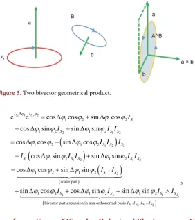
To calculate the geometric algebra product of the two exponents in Clifford translation with not coinciding exponent planes, _eIS1∆φ I φ1_eS22,

1 2

S ≠S , let’s first expand IS1 in original basis to get formulas for generators of Clifford transla-tion. If IS1=

γ

1 1B +

γ

2B2+

γ

3B3 then a part of geometrical product

1 2

eIS∆φ I φeS is:

(

)(

)

(

) (

)

(

)

(

)

(

)

(

)

1 2

1 2 1 2

1 1 2 2 3 3 1 1 2 2 3 3

1 1 2 2 3 3 3 2 2 3 1 1 3 3 1 2 2 1 1 2 3

3

S S

S S S S

I I

B B B B B B

B B B

I I I I I

γ γ γ β β β

γ β γ β γ β γ β γ β γ β γ β γ β γ β

= + + + +

= − + + + − + − + −

= − ⋅γ β − γ β× = ⋅ + ∧

(see Figure 3)

where γ and β are vectors dual to bivectors IS1 and IS2. Thus, the full product is:

2_{In the case of constant plane of Hamiltonian, it easily follows the Schrodinger equation of}

(7)

[image:7.595.233.516.72.390.2]

Figure 3. Two bivector geometrical product.

(

)

(

)

1 2

1

2 1 2

1 2 2

1 1 2 1 2

1 2 1 2

e e cos cos sin cos cos sin sin sin cos cos sin cos

cos sin sin sin

S S

I I

S

S S S

S S S S S

I

I I I

I I I

I I I I I

ϕ ϕ _ϕ _ϕ _ϕ _ϕ

ϕ ϕ ϕ ϕ

∆ = ∆ + ∆ + ∆ + ∆ = ∆ − ∆ − ∆ + ∆

(

)

( ) ( ) 1 2

1 2 1 2

scalar part

bivector part,expansion in no

1 2 1 2

1 2 1

n-orthonormal basis 2

,

1 2

,

cos cos sin sin

sin cos cos sin sin sin

S S S S

S S

S S S S

I I I I

I I

I I I I

ϕ ϕ ϕ ϕ

ϕ ϕ ϕ ϕ ϕ ϕ

∧ = ∆ + ∆ ⋅ + ∆ + ∆ + ∆ ∧   3

4. Transformations of Circular Polarized Electromagnetic

Fields

Now we have everything to retrieve action of Clifford translation generated by a Hamiltonian on general solution (4):

( )

( ) ( )

₍

₎

(

( ( ) ) ( ( ) )

)

3

3 3

0 3 0

e eS S eS S

t

I t t

t I t I I I t I I

I λ ω µ ω

 

 

−_ _ ∆

− ⋅ + ⋅

  ₊ r ₊ r

E H

 _



To make expressions simpler I will use notations

( )

3

t

I I

t ≡ 



 ,

(

)

(

t I I3 S

)

ω − ⋅ ≡r ϕ₊, and ω

(

t+

(

I I₃ _S

)

⋅ ≡r

)

ϕ₋. Then we get (see Sections 1.3

and 1.6 in [3] for multiplication details):

( )

₍

₎

(

)

(

)

(

( ) ( )

)

0 3 0

e e e

e e e e

S S

I t t I I

I t t I I t t I

I I ϕ ϕ ϕ ϕ λ µ λ µ + − + − − ∆ − ∆ − ∆ + + = − + + E H E H      

(

)

(

( )

)

(

( )

)

(

)

(

)

(

( )

)

(

( )

)

( )

(

)

(

)

(

)

(

( )

)

( )

(

)

(

( )

)

(

)

0 3 0

cos cos sin sin

sin cos cos sin

sin sin sin cos

cos sin sin sin

S

S S

I t t t t I I

I t t I t t I

t t I I I t t I

t t I t t I I

λ ϕ ϕ

ϕ µ ϕ

ϕ ϕ + + + + + − − − = − + ∆ − ∆ ⋅ − + ∆ + ∆ + ∆ ∧ − + ∆ + ∆ + ∆ ∧ E H E H E H             

3_{In the case}

1 2

S S

I =I we trivially have rotation of _eIS2ϕ2

(8)

DOI: 10.4236/***.2018.***** 711 Journal of Applied Mathematics and Physics Let’s take popular case of IS =B3=xˆˆy (plane orthogonal to zˆ axis) and

1 yzˆ ˆ

I_=B = (or I=B2=zxˆˆ, does not matter.) The above formula becomes:

(

)

(

( )

)

(

( )

)

( )

(

)

(

( )

)

( )

(

)

(

( )

)

(

( )

(

)

(

( )

)

0 3 0 1

2 3

1

2 3

cos cos sin cos

sin sin cos sin

cos cos sin cos

sin sin cos sin

I t t t t B

t t B t t B

t t t t B

t t B t t B

λ ϕ ϕ

ϕ ϕ

µ ϕ ϕ

ϕ ϕ + + + + − − − −  − + _ ∆ + ∆ + ∆ + ∆ + ∆ + ∆  + ∆ + ∆ _

E H  

 

It makes simpler if F₊ and F₋ are equally weighted, say both λ and μ are equal to one:

(

)

(

( )

)

(

)

(

( )

)

(

)

( )

(

)

(

)

(

( )

)

(

)

(

) ( )

(

( )

)

(

( )

)

( )

(

)

(

( )

)

0 3 0 1

2 3

0 3 0 1

2 3

cos cos cos sin cos cos

sin sin sin cos sin sin

2 cos cos cos sin cos

sin sin c

ˆ

os sin

z

I t t t t B

t t B t t B

I t t t t t tB

t t tB t t tB

ϕ ϕ ϕ ϕ

ω ω ω ω + + − − − − + + + +  +  − + _ ∆ + ∆ + ∆ + ∆  − + _ ∆ + ∆ + ∆ + + _ = ⋅ ∆ E E r H H         (6)

5. Action of Polarization States on Observables

Since a state in the described formalism is operator that gives the result of mea-surement when acting on observable, which can be any element of geometric al-gebra G3, the following is detailed description of the case when the element in

parenthesis of the (6) expression acts on some bivector. Such operation is gene-ralization of the Hopf fibration and rotates the bivector in three dimensions.

Denoting4_:

( )

(

)

(

( )

)

( )

(

)

(

( )

)

, 1 2 3

1 1 2 2 3 3

cos cos sin cos

sin sin cos sin

eI

t t t t t tB

t t tB t t tB

B B B ωψ

ω

α β

β

∆ + ∆ + ∆ + ∆ ≡ + + + ≡      where

(

)

, 1 1 2 2 3 3

Iω =

γ

B +

γ

B +

γ

B

( )

(

)

( )

(

)

(

( )

)

1

2 2 2

sin cos

sin cos sin

t t t

t t t t t

ω γ ω ∆ = ∆ + ∆   

( )

(

)

( )

(

)

(

( )

)

2

2 2 2

sin sin

sin cos sin

t t t

t t t t t

ω γ ω ∆ = ∆ + ∆   

( )

(

)

( )

(

)

(

( )

)

3

2 2 2

cos sin

sin cos sin

t t t

t t t t t

ω γ ω ∆ = ∆ + ∆   

4_{Easy to see that the left-hand side is unit value element of}

3

(9)

( )

(

)

(

)

1

cos cos t t cos t

ψ ₌ − _ _∆ ω

and taking a bivector operand (observable) c B1 1+c B2 2+c B3 3 we get the result

of measurement, action of the state on observable (see [3], [4] for details):

(

)

(

) (

)

(

)

(

)

(

)

(

)

(

) (

)

(

)

(

)

(

)

(

)

(

) (

)

(

)

, ,

1 1 2 2 3 3

2 2 2 2

1 1 2 3 2 1 2 3 3 1 3 2 1

2 2 2 2

1 3 1 2 2 2 1 3 3 2 3 1 2

2 2 2 2

1 1 3 2 2 2 3 1 3 3 1 2 3

e e

2 2

I I

c B c B c B

c c c B

ωψ ωψ

α β β β β β αβ β β αβ

αβ β β α β β β β β αβ

β β αβ β β αβ α β β β

− ₊ ₊

 

= _ + − + _+ − + +

 

+ + + _ + − + _+ −

 

+ − + + + _ + − + _

 

( )

(

)

(

( )

)

(

)

(

)

( )

(

)

(

( )

)

(

)

(

)

( )

(

)

(

( )

)

(

)

1 2 3 1

1 2 3 2

2 3 3

cos 2 sin 2 cos 2 sin 2

sin 2 cos 2 cos 2 sin 2

sin 2 cos 2

c t t c t t c t t B

c t t c t t B

ω ω

= − ∆ − ∆

+ + ∆ − ∆

+ ∆ + ∆

 

One interesting remark. If the observable belongs only to the B1 plane, that’s

3

2 0

c =c = , the result of measurement has only components in B1 and B2,

projections of the value c1 due to rotation with angular velocity 2ω around the ˆ

z axis.

6. Polarization States Acting on Multiple Observables

The core of quantum computing should not be in entanglement as it understood in conventional quantum mechanics, which only formally follows from repre-sentation of the many particle states as tensor products of individual particle states and not supported by really operating physical devices. The core of quan-tum computing scheme should be in manipulation and transferring of sets of states as operators decomposed in geometrical algebra variant of qubits (g-qubits), or four-dimensional unit sphere points, if you prefer. Such operators can act on observables, particularly through measurements. From the recent calculation we realize that the action of state, which depends on

( )

t r, , on an observable can be done only if observable is defined at the same point

( )

t r, where the state is defined [5]. In this way quantum computer is an analog com-puter keeping information in sets of objects with infinite number of degrees of freedom, contrary to the two value bits or two-dimensional Hilbert space ele-ments, qubits.

Thus, if we have a state

( , ,S) ( ( ) ( ) ( ), , , ,S , )

S I t t I t

I g _{α β} g _α _β

α

+

β

≡ = _r _r _r

as in the case of polarization defined states, it becomes a state acting on a set of observables if the latter are defined at some given points:

( ) ( )

( n n, ,C n n, ) 0

(

,

)

(n n, ) 1 02

(

,

)

, 1, ,

n c t I t n n C t n n

c = c =c t +I _r −c t n= N

r r r r 

(10)

Figure 4. Decoding of g-qubit message.

(

) (

)

(

)

(

) (

)

( ) ( ) ( )

( )

(

) (

)

( ) ( ) ( )

( )

(

) (

)

( ) ( ) ( )

( )

(

) (

)

1 1 1 1 1 1

1 , , , , , 1 1

, , , , ,

1 , , , , ,

, , , , , , , , , ,

d d d d

d d S

S

S N N N N S N N

N t t I t

N N

t t I t

n N

n n

n t t I t

g t t I t g t t I t

g g g t t t

g t t t

α β

α β α β

δ δ

= =

≡ = − − +

+ − −

= − −

∫∫

∑ ∫∫

r r r

r r r r r r

r r r

 



This formula for g1gN bears clear physical and geometrical sense, con-trary to conventional quantum mechanics definition following formally from tensor product which does not have good physical interpretation but is the root of entanglement-based quantum computing.

The formula also prompts how quantum encryption decoding can be effec-tively implemented with the bivector value security key (see Figure 4).

The formula can also be applied to challenging area of anyons in three dimen-sions.

7. Conclusion

Two seminal ideas—variable and explicitly defined complex plane in three di-mensions, and the G3

+_states5_{as operators acting on observables—allow to put} forth comprehensive and much more detailed formalism appropriate for quan-tum mechanics in general and particularly for quanquan-tum computing schemes. The approach may be thought about, for example, as a far going geometric alge-bra generalization of some proposals for quantum computing formulated in terms of light beam time bins, see [6], [7], but giving much more strength and flexibility in practical implementation.

References

[1] Soiguine, A. (2017) Quantum Computing with Geometric Algebra. Future Tech-nologies Conference, 28-30 November 2017, Vancouver, Canada.

[2] Soiguine, A. (1996) Complex Conjugation-Relative to What? Clifford Algebras with Numeric and Symbolic Computations, Boston, Birkhauser, 284-294.

[3] Soiguine, A. (2015) Geometric Phase in Geometric Algebra Qubit Formalism. LAMBERT Academic Publishing, Saarbrucken.

[4] Soiguine, A. (2015) Geometric Algebra, Qubits, Geometric Evolution, and All That.

http://arxiv.org/abs/1502.02169

[5] Soiguine, A. (2016) Anyons in Three Dimensions with Geometric Algebra.

http://arxiv.org/abs/1607.03413

[6] Humphreys, P.C., et al. (2013) Linear Optical Quantum Computing in a Single

Spa-5_{Good to remember that “state” and “wave function” are (at least should be) synonyms in}

(11)

tial Mode. Physical Review Letters,111, 150501-1-150501-5.

https://doi.org/10.1103/PhysRevLett.111.150501

[7] Kok, P., et al. (2007) Linear Optical Quantum Computing with Photonic Qubits.

Reviews of Modern Phys.ics 89, 135-174.