FFmpeg based Coding Efficiency Comparison of H 264/AVC, H 265/HEVC and VP9 Video Coding Standards for Video Hosting Websites

FFmpeg based Coding Efficiency Comparison of

H.264/AVC, H.265/HEVC and VP9 Video Coding

Standards for Video Hosting Websites

Jani Pavliˇc

Faculty of Electrical Engineering and Computer Science Koroška cesta 46

Jernej Burkeljca

Faculty of Electrical Engineering and Computer Science Koroška cesta 46

ABSTRACT

This paper describes the impact of different camera movements, object motions and scene details on the video compression factor by using FFmpeg to compare the efficiency of Standards VP9, H.264 and H.265 at bit rates recommended for video hosting websites. The study showed that H.265 outperformed H.264 and VP9 in all six cases, where compression efficiency depended highly on the video content, as well as Video Coding Standard. FFmpeg showed to be an usable alternative for assessing objective visual quality.

General Terms

Compression factor, lossy video compression, objective visual quality measurement

Keywords

Video compression efficiency, FFmpeg, H.264, H.265, VP9, PSNR, SSIM

1. INTRODUCTION

File size and bit rate are some of the major issues concerning digital video and the leading motivating factor for video compression. The latter involves algorithms which reduce the number of bits and attempt to keep relatively similar visual perception. Such algorithms are defined by various video compression Standards which improve compression efficiency, or so-called compression factor [24] [27].

Numerous experiments have established improved compression efficiency in line with the development of Video Compression Standards. Researchers have used the Bjøntegaard model to calculate and compare objective visual quality differences between Rate-Distortion (RD) curves at different bit rates [2]. Ponlatha and Sabeenian [24] predicted 25% improvement of the H.265/MPEG-HEVC Standard compared to H.264/MPEG-AVC. Kufa and Kratochvil [13] demonstrated the H.265 encoder to be 25% more efficient than VP9, while results by Grois et. al [10] describe that H.265 outperformed VP9 and H.264 by 43,3% and 29,3% respectively.

Despite various attempts to test video compression efficiency by using a wide range of bit rates and video encoders, little attention has been paid to the narrower scope of video compression efficiency at bit rates suitable specifically for video hosting websites relative to different clip content. In addition, results in prior experiments have been obtained mostly by using the MSU Quality Measurement Tool [16], while alternatives such as FFmpeg exist [5]. Lastly, other studies have not considered compression factor, which can be perceived very naturally , since a positive correlation exists between the factor and the compression efficiency [27].

The aim of this study is to compare compression factors of Standards H.264 (also known as AVC or MPEG-4 part 10), H.265/HEVC and VP9 at bit rates recommended for videos on video sharing websites at certain objective visual quality in correlation with video content (camera movement, object motion, scene details). The previous study [28] pointed out that 36% of all respondents use the open source software FFmpeg for encoding. Despite the useage of the aforementioned tool for encoding purposes, it has not been established for objective visual quality assessment. In the present study, FFmpeg encoders were used for video compression, and FFmpeg filters for assessing objective visual quality. Although FFMPEG 4.0 supports the newest Standard AV1, it was not taken into account in this paper since initial tests showed extremely slow encoding time (475 times slower than H.265) [22] and, therefore, poor usability for large scale deployment.

This paper is organized as follows. A brief overview of concepts regarding video compression, Video Coding Standards and objective visual quality is given in Sections 2 and 3, followed by a description of an experimental procedure based on FFmpeg in Section 4. Results are presented and explained in Section 5. Finally, the conclusion is given in Section 6.

2. VIDEO COMPRESSION

research on video compression at bit rates suitable for video hosting websites. Therefore, this study is focused on the widely researched Video Coding Standards H.264 / AVC, H.265 / HEVC and VP9, pointed out by many researchers, e. g. [11, 15, 13], who conducted experiments to calculate codec efficiency.

Salomon and Motta [27] showed a simple calculation table indicating that a video with HD resolution (1920x1080) at 60 frames per second is needed to be sent with a bit rate of 2,985,984,000 bits/sec. Due to limited bandwidth and storage space, lossy video compression plays a significant role in reducing the number of bits and achieving similar visual perception [24].

Ponlatha and Sabeenian [24] defined compression as reducing insignificant redundancies which can be divided into four types: Perceptual, temporal, spatial and statistical. They refer to reducing details with higher frequencies, similarities between successive frames and binary codes without affecting the visual perception. The coding process can be implemented within one frame (intra prediction) and between two or more frames (inter prediction), where each frame is divided into smaller units called blocks or macroblocks.

In terms of video compression, changes between video frames play an important role. They can be caused by object motion, camera movement, uncovered regions and lighting changes. While uncovered regions and lighting changes can produce new information, other changes are predictable and calculable based on previous encoded frames [25]. According to Mengzhe et al. [15], there exists a negative correlation between scene complexity and visual quality. The present research does not consider concepts of video complexity, as its focus is on the changes between video frames of each clip, and the correlation with compression efficiency.

A further explanation of video compression concepts and Video Coding Standards is given in literature by Richardson [25] and Salomon & Motta [27].

2.1 H.264 / AVC

H.264 or Advanced Video Coding (AVC) was developed and Standardized collaboratively by the International Telecommunication Union (ITU-T) Video Coding Expert Group (VCEG) and ISO / IEC Moving Picture Experts Group (MPEG). H.264 is currently one of the most established Standards. Taking into account the Unisphere research [28], 78% of all survey respondents chose the H.264 Standard as their main Video Encoding Standard. Others [29] analyzed file types served by websites with video content and saw H.264 in 53% of cases, despite being superceeded by newer Standards many years ago. Wiegand et al. [38] highlight the main features of the Standard in relation to prior Video Coding Standards. In terms of motion compensation, H.264 supports more flexible block sizes (4 x 4 – 16 x 16) and quarter sample accurate motion compensation. It also differs from its predecessors by using a large number of previously decoded frames to predict the values of an incoming frame.

Transformation and quantization operations are further improved in the sense of reducing calculations’ processing while maintaining the transformation accuracy and eliminating unimportant data to achieve higher compression efficiency [26]. Another important feature is a de-blocking filter, which can improve visual quality by reducing blocking artifacts [38]. H.264/AVC includes two entropy coding methods, called CAVLC (Context-Adaptive

Variable-Length Coding) and CABAC (Context-Adaptive Binary Arithmetic Coding), as an upgrade of VLC (Variable-Length Codes) for mapping transformed coefficient levels and improving coding efficiency [14, 38].

According to Wieagand at al. [38] the combination of mentioned features can achieve approximately 50% bit rate savings compared to prior Standards.

2.2 H.265 / HEVC

High Efficiency Video Coding (HEVC) or H.265, developed jointly by VCEG and MPEG, is a successor to the H.264. In terms of video compression efficiency, H.265 can achieve approximately a 50% bit rate savings in relation to prior Standards, especially for high-resolution video [30].

As well as prior Standards, H.265 is also based on the hybrid approach of the inter / intra prediction coding processes, with a redefined structure of blocks. Macroblock is renamed in a so-called Coding Tree Unit (CTU), the size of which can be larger than the traditional macroblock. The CTU consists of a Luma Coding Tree Block (CTB) and the chroma CTBs, where the size is either 16, 32 or 64 squared samples. CTBs are further split into coding blocks with a minimum size of 4 x 4 samples [18, 30]. Variable size blocks provide more flexibility in adapting to video scene content. Smaller block sizes are used in areas with more details, while larger blocks can be used in areas with fewer details (e.g. sky) [34].

Another novelty is Advanced Motion Vector Prediction (AMVP), which takes into account the most suitable motion vectors of the reference frames. The precision of motion compensation is up to a quarter-sample. Similar to H.264, multiple reference frames are used for either uni-predictive or bi-predictive coding [30]. An important difference between the two is encoding within one frame, as H.265 supports 35 directions or prediction modes, while H.264 supports only 9 [23]. In line with encoding complexity, H.265 expands the search space for intra prediction modes and therefore burdens computation and increases coding time [34].

2.3 VP9

Due to the need for efficient open-source video codecs, Google developed VP9 (the successor of VP8) as a part of the WebM project to which anyone can contribute freely [17, 37].

Mukherjee et al. [17] outlined the main tools included in VP9. Among others are the so-called Super-Blocks (SB) with the maximum size of 64 x 64 blocks, that can be broken further down into 4 x 4 blocks in 13 different endpoint block sizes. The codec supports 10 intra prediction modes and 4 inter prediction modes for calculating the motion vectors. Each frame can have up to three reference frame buffers selected. Alternative reference frames, which are never displayed, can be used to improve coding efficiency. The encoder can choose the precision to be between a quarter sample or one eighth of a sample. Similar to H.264 and H.265, the loop filter is used to eliminate blocking artifacts.

2.4 Compression factor

The compression Factor (F) is defined as a ratio between the size of the input stream and the size of the output stream [27]. Instead of the size of the input and output stream, it is possible to use bit Rates (R) of uncompressed and compressed videos as follows:

F=R_Runcompressed

compressed (2.1)

For F > 1 a positive correlation applies. The greater the compression factor, the better the compression [27].

2.5 FFmpeg

FFmpeg is an open-source multimedia framework intended mainly for encoding and decoding. It supports a wide range of different coding options and filters. FFmpeg is supported by Windows, Linux and macOS operating systems [5, 6, 7].

In the present study, FFmpeg was used for encoding and evaluating the objective visual quality of different videos. Further information about objective visual quality and the experimental procedure is given in the following sections.

3. OBJECTIVE VISUAL QUALITY

Visual quality can be objective or subjective. Since subjective visual quality depends on individuals, the objective one is usually taken into account [19]. An important advantage of objective visual quality measurements is the repetability of research[32]. The measurements are divided into three categories: Full reference, reduced-reference and no-reference [40]. This paper is focused on the full-reference category, as it includes a comparison of a compressed frame to a reference (uncompressed or original) frame.

Objective measurement algorithms are used by developers of Video Coding Standards. According to existing research [12, 25, 40], Peak Signal-to-Noise Ratio (hereinafter PSNR) and Structural Similarity Index (hereinafter SSIM) are the most commonly used measurements.

3.1 PSNR

PSNR refers to the ratio between the maximum possible value of a signal and the Mean Squared Error (hereinafter MSE) between the original and distorted (compressed) frame (equation 3.1) [19, 25]. It is expressed in decibels, where higher values refer to a greater similarity between frames and, consequently, better visual quality of the compressed frame [27]. By contrast, smaller values indicate a high numerical difference between two frames [12].

Equation 4.1 shows how to calculate the PSNR value. The maximum value of the signal is2n_{−1, where}

nrepresents the number of bits per pixel [25]. MSE is a comparison between pixels’ values in an original and degraded frame. It can be calculated as in equation 3.2 [19].

PSNR=

20

∗

log

(

n₋₁

√

M SE

)

MSE=_mn1

m−1

X

0

n−1

X

0

[

f

(

i, j

)

−

g

(

i, j

)]

Wheref– is the matrix data of an original image;g– is the matrix data of a degraded image;m– is the numbers of rows of pixels of the frame; (i– is the index of that row);n– is the number of columns of pixels of the frame; (j– is the index of that row) [19]. The PSNR value does not have an absolute meaning. The values are most useful in comparing efficiency between various Video Coding Standards. For instance, MPEG committee uses the difference 0,5 dB as a visible improvement of coding optimization [27].

3.2 SSIM

SSIM measures the similarity between two images or frames. It is considered to be more consistent with human perception than PSNR. During the examination of a blurred image, the results of SSIM measurements considered the image to be bad quality, whereas results from PSNR did not show any quality flaws compared to the original image [20].

Because of the correlation with human perception, SSIM has recently been applied to image and video compression analysis. It takes into account structural changes of frames, such as blur and lossy compression [42]. Figure 1 shows two examples of structural change.

Fig. 1. Original image, blurred image, compressed image [42]

Equation 3.3 shows the calculation of the SSIM index. It measures the similarity of three different elements – luminance (l), contrasts (c) and structure (s), where parameters (x) and (y) refer to images x and y [42].

SSIM (x,y) = l(x,y) c(x,y) s(x,y) (3.3)

SSIM holds a value from an interval of[0,1], where0is the worst quality and1the best [32].

The concepts of all equations (3.1, 3.2 and 3.3) are important for understanding the variables of the measurements. Nevertheless, this paper does not focus on mathematical statements and proof of concepts, since FFmpeg was used to obtain video quality results.

4. EXPERIMENTAL PROCEDURE

The present study involved an experiment comparing the compression efficiency or compression factors of Standards H.264, VP9 and H.265 at a neglible difference of objective visual quality as well as different bit rates settings, both suitable for video hosting websites. The experiment was conducted on six different video clips using FFmpeg libraries x264, x265 and libvpx for encoding, which conform to H.264, H.265 and VP9 Standards respectively [8]. In addition, FFmpeg filters were used to obtain the PSNR and SSIM values [7].

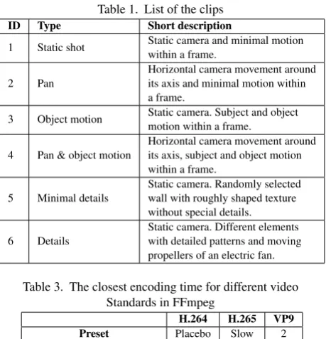
A total of 6 video clips of 10 seconds duration were captured in a raw video format (1920 x 1080 px, 25 fps, 10 bit, YUV 4:2:2). The first 4 clips differed in camera movement and object motion, while the last 2 clips varied in the details within a scene. The types and descriptions of clips are given in Table 1. The visual example of a frame within clip no. 3 is shown in Figure 2.

Fig. 2. An example of a random frame within clip 3

Initially, the clips were encoded using the x264 encoder, at an average bit rate of approximately 8000 kbit/s. This follows the guidelines of the popular video sharing websites mentioned in Table 2. Each video was then encoded in turn with the other two encoders by changing the target average bit rate settings until a similar objective visual quality was achieved. The assessment consisted of comparing each reference frame with the compressed one and obtaining an average PSNR and SSIM value using the FFmpeg.

In this case of compression with different video Standards, it was not possible to achieve equivalent objective quality. Therefore, it was necessary to aim for an optimal approximation. To this end, the accuracy of PSNR was rounded to one decimal place of its value for each encoded video. To ensure equivalent objective quality of a video encoded by different Standards, each rounded PSNR value had to be equal (e.g. 47,2 dB for clip 1 as shown in Table 4). This method is more accurate than the recommended accuracy defined by the MPEG committee, as described in Section 3. The same procedure was applied when comparing SSIM. In this case, the values were rounded to two decimal places (e.g. 0,99 for clip 1 as shown in Table4).

Encoding and evaluating video quality in FFmpeg was done through the command line as shown in Figure 3. Default profile and level settings were used in the encoding process. Those settings adjust automatically depending on other input parameters. The resolution and frame rate did not have to be specified, since the

Table 1. List of the clips ID Type Short description

1 Static shot Static camera and minimal motion within a frame.

2 Pan

Horizontal camera movement around its axis and minimal motion within a frame.

3 Object motion Static camera. Subject and object motion within a frame. 4 Pan & object motion

Horizontal camera movement around its axis, subject and object motion within a frame.

5 Minimal details

Static camera. Randomly selected wall with roughly shaped texture without special details. 6 Details

Static camera. Different elements with detailed patterns and moving propellers of an electric fan.

Table 3. The closest encoding time for different video Standards in FFmpeg

H.264 H.265 VP9 Preset Placebo Slow 2

Average coding speed (fps) 1.1 0.90 1.2

value of these parameters matched automatically. As FFmpeg does not support an option for constant bit rate settings, it was limited by applying options for maximum and minimum bit rate.

It is important to point out that the objective visual quality depends on preset settings that determine the coding process speed at the expense of compression efficiency. In order to minimize the impact of that factor, it was crucial to equalize the coding speed as much as possible. For this purpose, a pre-experiment was conducted to test the coding speed with different preset settings. Results of the pre-experiment for a randomly selected video are shown in Table 3. According to the results, preset settings "placebo" and "slower" were used in x264 and x265 respectively1 _{and, in the}

case of libvpx, a preset setting with the value 22_{. Coding speed}

settings were considered as a limitation since x264 used the slowest possible level, which allowed better use of available compression modes. The coding speed experiment was performed on a computer with an Intel i7 processor with the frequency of 3,40 GHz, 32 GB RAM and GeForce GTX 650 1 GB.

Finally, in the main experiment of this paper, the compression factors were calculated for all cases. Based on the results, the compression efficiency was determined, and bit rate savings were calculated for each Standard. The interpretation of results is given in the following section.

5. RESULTS AND DISCUSSION

The majority of data obtained in previous studies showed H.265 to be more efficient than others [24, 11, 13]. This was confirmed in this paper as H.265 outperformed both H.264 and VP9 in all cases (see 4). Nevertheless, differences between compression

1_{Coding speeds are defined with 10 different levels, where "placebo" is the}

slowest and "slower" is two levels faster.

2_{Coding speed values for libvpx range from 1 to 5, where 1 is the slowest}

Table 2. Technical video recommendations for the resolution 1920 x 1080 px [39, 35, 4, 31]

Youtube Vimeo Daily motion Twitch Container MP4 MP4 and others MP4 and others MP4 and others.

Standard H.264 H.264 / ProRes / HEVC H.264 H.264

Bit rate(Mbit/s) 8 10 – 20 6 – 8 up to 10

Frame rate(fps) 24 – 60 23.98 – 60 24 – 50 up to 60

Video platforms are selected according to the list of the website eBiz [9]. .

Fig. 3. Sample commands for encoding and obtaining PSNR & SSIM values

factors varied for each video clip, indicating the dependence of the compression efficiency on the content of the video.

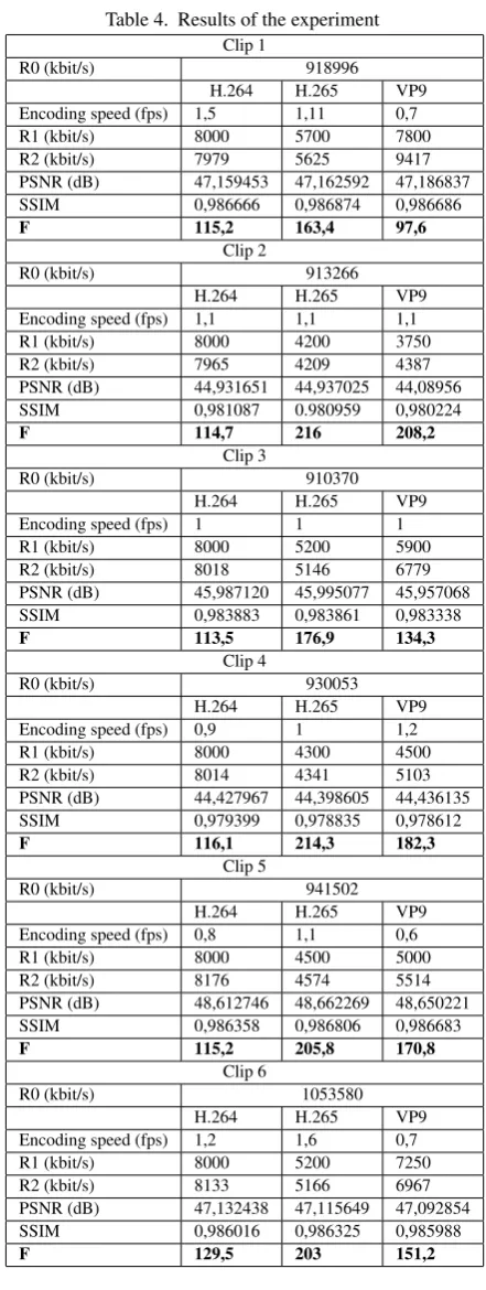
Data in Table 4 show results obtained using FFmpeg. Every clip was first encoded by x264 at a target bit rate (R1) 8000 kbit/s. Since the actual average bit rate deviated from the target, it was marked as R2 in all cases. As mentioned in Section 4, bit rate changes were made until the PSNR and SSIM values were equal after rounding to one and two decimal places respectively. Both measurements always changed in accordance with compression, therefore, they both seem to be a good method to measure quality in terms of video compression.

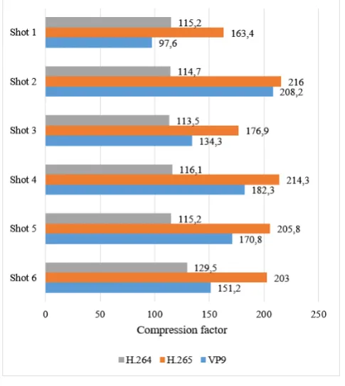
Compression factors were calculated for each clip and Standard separately, as shown in equation (2.1), where R0 is a bit rate of an uncompressed video and R2 is an average bit rate of a compressed video. The compression factor differences can be seen in 4. The chart does not serve to compare the compression efficiency between two different clips, as they have different objective visual quality. It is usable at most to compare the differences in coding efficiency of different Standards within one clip.

Compression factors of videos coded with x264 are quite similar, since the same target bit rate was used for each clip. Nevertheless, H.264 returned the worst compression factor in 5 out of 6 clips. This means it was the least effective in terms of video compression.

In most cases, VP9 turned out to have a better compression factor than H.264, with an exception in the static case 1. In the latter, VP9 had the worst compression factor. This could be due to an extended use of reference frames in H.264, e.g. 5 frames in the profile Main [38, 25], whereas VP9 can use up to 3 reference frames for motion compensation [17]. Although using multiple reference frames increases coding time, it also has an impact on compression efficiency in conjunction with some other modes [25]. In the case of the present study where the settings for slow coding time were used, encoders had enough time to search for different blocks within different frames in order to find the best match.

Even though H.265 was the most effective in every clip, VP9 came quite close in the case of clip 2. It turned out the efficiency of the two Standards was just slightly different in the case of

Fig. 4. Compression factor

camera motion and uncovered regions. Most likely, the reason lies in the process of uncovering new regions by panning, which requires encoding of new information within blocks. Therefore, the advantages of H.265 were less apparent in motion compensation.

In other cases, the difference in compression efficiency between H.265 and VP9 was more evident. Despite the incomparable difference of compression factor between two or more different clips for each Standard, it was possible to calculate bit rate savings between them. The bit rate savings are shown in Table 5. In the parenthesis of each cell, a Standard that outperformed its opponent is given. In general, the highest variation of bit rate savings was discovered between H.264 and VP9. It means the difference in compression efficiency of the two depended highly on the clip content. Therefore, one should be careful when choosing one Standard over the other.

Table 4. Results of the experiment

Clip 1

R0 (kbit/s) 918996 H.264 H.265 VP9 Encoding speed (fps) 1,5 1,11 0,7 R1 (kbit/s) 8000 5700 7800 R2 (kbit/s) 7979 5625 9417 PSNR (dB) 47,159453 47,162592 47,186837 SSIM 0,986666 0,986874 0,986686

F 115,2 163,4 97,6

Clip 2

R0 (kbit/s) 913266 H.264 H.265 VP9 Encoding speed (fps) 1,1 1,1 1,1 R1 (kbit/s) 8000 4200 3750 R2 (kbit/s) 7965 4209 4387 PSNR (dB) 44,931651 44,937025 44,08956 SSIM 0,981087 0.980959 0,980224

F 114,7 216 208,2

Clip 3

R0 (kbit/s) 910370 H.264 H.265 VP9 Encoding speed (fps) 1 1 1 R1 (kbit/s) 8000 5200 5900 R2 (kbit/s) 8018 5146 6779 PSNR (dB) 45,987120 45,995077 45,957068 SSIM 0,983883 0,983861 0,983338

F 113,5 176,9 134,3

Clip 4

R0 (kbit/s) 930053 H.264 H.265 VP9 Encoding speed (fps) 0,9 1 1,2 R1 (kbit/s) 8000 4300 4500 R2 (kbit/s) 8014 4341 5103 PSNR (dB) 44,427967 44,398605 44,436135 SSIM 0,979399 0,978835 0,978612

F 116,1 214,3 182,3

Clip 5

R0 (kbit/s) 941502 H.264 H.265 VP9 Encoding speed (fps) 0,8 1,1 0,6 R1 (kbit/s) 8000 4500 5000 R2 (kbit/s) 8176 4574 5514 PSNR (dB) 48,612746 48,662269 48,650221 SSIM 0,986358 0,986806 0,986683

F 115,2 205,8 170,8

Clip 6

R0 (kbit/s) 1053580 H.264 H.265 VP9 Encoding speed (fps) 1,2 1,6 0,7 R1 (kbit/s) 8000 5200 7250 R2 (kbit/s) 8133 5166 6967 PSNR (dB) 47,132438 47,115649 47,092854 SSIM 0,986016 0,986325 0,985988

F 129,5 203 151,2

Table 5. Bit rate savings

H.264 vs. H.265 H.264 vs. VP9 VP9 vs. H.265 clip 1 30% (H.265) 15% (H.264) 40% (H.265) clip 2 47% (H.265) 45% (VP9) 4% (H.265) clip 3 36% (H.265) 15% (VP9) 24% (H.265) clip 4 46% (H.265) 36% (VP9) 15% (H.265) clip 5 44% (H.265) 33% (VP9) 17% (H.265) clip 6 36% (H.265) 14% (VP9) 26% (H.265)

subject motion in both clips, which was not completely consistent. It differed in body parts’ speed and in a way of overlapping or uncovering the scene. Another reason might be the coding speed, which, in this case, was set to the best (slowest) level for encoder x264 (Section 4).

Although VP9 and H.265 were more efficient than H.264 in clips 5 and 6, the bit rate savings versus H.264 deteriorated for the detailed scene (clip 6). This implies high variability of the two Standards according to details within a scene. As noted in Section 2, H.265 and VP9 support more flexible block sizes. It can be inferred that larger block sizes were used in clip 5 since there were fewer details. Consequently, more blocks, motion vectors and calculations were applied in the case of clip 6, which resulted in more data and lower factors.

6. CONCLUSION

Prior research on the video compression efficiency of Video Compression Standards was based on calculating the differences between rate-distortion curves and showing generally improved compression efficiency [2, 24, 11, 13]. This study was focused on recommended video bit rates for video hosting websites. It considers comparison of compression efficiency expressed in compression factor on six video clips differing in camera movement, object motion and details within a scene. The open source tool FFmpeg was used for the needs of encoding and objective visual quality assessment.

It was concluded that H.265 returned the best compression efficiency in all cases, while H.264 turned out to be the least efficient. Nevertheless, results were highly dependent on the content of the video clips, and always returned obvious difference between two Standards. That confirms the expected correlation between compression efficiency and types of video.

The outcome of the research gives an insight into understanding the compression efficiency depending on the type of video clip and the particular video Standard, the use of an alternative and cost-effective video quality assessment tool, and for publishing video content on video hosting websites.

Based on the present experiment, it can be stated that H.265 is the most recommended for video hosting websites, in terms of compression efficiency, followed by VP9. Nevertheless, limitations such as encoding-decoding time efficiency, computational burden and work flow modifications must be taken into account. Even though H.264 turned out to have the worst compression factor out of the compared Standards, it can be much more efficient in other areas, such as coding and decoding speed, which also explains why its use has not declined much even though newer Standards exist.

various advanced camera motion or additional graphic elements. AV1 was not taken into account in this study, since it is still under development. Nevertheless, the aforementioned codec represents a real competitor to H.265 in the future, due to its support by many leading tech organizations striving for cost-effective video coding [1]. It would be interesting to compare the efficiency of the AV1 and H.265 Standards by using the procedure described in this paper. In terms of software, FFmpeg can be used further for assessments of objective visual quality for researchers as well as distributors of audiovisual web content.

7. AKNOWLEDGMENTS

The authors gratefully aknowledge the assistance and support of Mitja Cvetko in setting up and conducting the experiment used in this research.

8. REFERENCES

[1] Alliance for open media. 2018. The Big Picture. Available at: https://aomedia.org/about/ [5. 6. 2018].

[2] Bjøntegaard, G. 2001. Calculation of average PSNR diferences between RDcurves. Technical Report VCEG-M33, ITU-T SG16/Q6, Austin, Texas, USA.

[3] Cisco. 2017. Cisco Visual Networking Index: Forecast and Methodology, 2016-2021. Available at: https://www.cisco.com/c/en/us/solutions/collateral/service- provider/visual-networking-index-vni/complete-white-paper-c11-481360.html [30. 5. 2018].

[4] Daily motion. 2018. Video Specifications. Available at: https://faq.dailymotion.com/hc/en-us/articles/115008879507-Video-Specifications [12. 9. 2018].

[5] FFmpeg. About FFmpeg. Availableat: https://ffmpeg.org/about.html [30. 10. 2018].

[6] FFmpeg. FFmpeg Documentation. Available at: https://ffmpeg.org/ffmpeg.html [23. 10. 2018].

[7] FFmpeg. FFmpeg Filters Documentation. Available at: https://ffmpeg.org/ffmpeg-filters.html [23. 6. 2018].

[8] FFmpeg. General Documentation. Available at: https://www.ffmpeg.org/general.html [23. 9. 2018].

[9] The eBusiness Guide. 2018. The 15 Most Popular Video Websites | May 2018. Available at: http://www.ebizmba.com/articles/video-websites [30. 5. 2018]. [10] Grois, D., Marpe, D., Mulayoff, A., Hadar, O. 2013.

Performance Comparison of H.265/MPEG-HEVC, VP9, and H.264/MPEG-AVC Encoders. 2013 Picture Coding Symposium.

[11] Grois, D., Nguyen, T., Marpe, D. 2016. Coding Efficiency Comparison of AV1/VP9, H.265/MPEG-HEVC, and H.264/MPEG-AVC Encoders. Picture Coding Symposium (PCS).

[12] Hore, A., Ziou, D. 2010. Image Quality Metrics: PSNR vs. SSIM. 20th International Conference on Pattern Recognition. [13] Kufa, J., Kratochvil, T. 2015. Comparison of H.265

and VP9 Coding Efficiency for Full HDTV and Ultra HDTV Applications. Radioelektronika, 2015 25th International Conference.

[14] Marpe, D., Schwarz, H., Wiegand, T. 2003. Context-Based Adaptive Binary Arithmetic Coding in the H.264/AVC Video Compression Standard. IEEE TRANSACTIONS ON

CIRCUITS AND SYSTEMS FOR VIDEO TECHNOLOGY, VOL. 13, NO. 7, JULY 2003.

[15] Mengzhe, L., Xiuhua, J., Xiaohua, L. 2015. Analysis of H.265/HEVC, H.264 and VP9 Coding Efficiency Based on Video Content Complexity. Computer and Communications (ICCC), 2015 IEEE International Conference.

[16] Vatolin, D., Moskvin, A., Petrov, O., Putilin, S., Grishin, S., Marat, A., Osipov, G. 2018. MSU Video Quality Measurement Tool. Available at: http://www.compression.ru/video/ [9. 11. 2018].

[17] Mukherjee, D., Bankoski, Jim., Grange, A., Han, J., Koleszar, J., Wilkins, P., Xu, Y., Bultje R. 2013. The latest open-source video codec VP9 - An overview and preliminary results. 2013 Picture Coding Symposium (PCS).

[18] MulticoreWare. HEVC/H.265 Explained. Available at: http://x265.org/hevc-h265/ [18. 6. 2018].

[19] National Instruments. 2013. Peak Signal-to-Noise Ratio as an Image Quality Metric. Available at: http://www.ni.com/white-paper/13306/en/ [3. 7. 2018].

[20] National Instruments. 2016. What’s New in NI Vision Development Module 2011. Available at: http://www.ni.com/white-paper/12956/en/ [3. 7. 2018]. [21] Ohm, J., Sullivian, G. J., Schwarz, H., Thiow Keng Tan,

Wiegand, T. 2010. Comparison of the Coding Efficiency of Video Coding Standards – Including High Efficiency Video Coding (HEVC). IEEE transactions on circuits and systems for video technology, vol. 22, no. 12, 2010.

[22] Ozer, J. 2018. Time to start Testing: FFmpeg Turns 4.0 and Adds AV1 Support. Available at: http://www.streamingmedia.com/Articles/Editorial/Featured- Articles/Time-to-Start-Testing-FFmpeg-Turns-4.0-and-Adds-AV1-Support-127685.aspx [3. 7. 2018].

[23] Patel, D., Lad, T., Shah, D. 2015. Review on Intra-prediction in High Efficiency Video Coding (HEVC) Standard. International Journal of Computer Applications (0975 – 8887). Vol. 132 – No. 13.

[24] Ponlatha, S., Sabeenian, R., S. 2013. Comparison of Video Compression Standards. International Journal of Computer and Electrical Engineering, Vol. 5, Å˘at. 6, , pages 549 – 554. [25] Richardson, I. E. G. 2003. H.264 and MPEG-4 Video

compression, UK Wiley.

[26] Saif, I. M., Zekry, A. 2015. Implementing Lossy Compression Technique for Video Codecs. International Journal of Computer Applications (0975 – 8887), Vol 131 – No. 7.

[27] Salomon, D., Motta, G. 2010 Handbook of data compression. 5th ed. Springer London Dordrecht Heidelberg New York, 2010, pages 1–23, 463–466, 480–503, 855–927.

[28] Siglin, T. 2018. Real-world HEVC insights: Adoption, implications, and workflows. Streaming Media magazine. [29] Sillars, D. 2018. Video Playback On The Web:

The Current State Of Video (Part 1). Available at: https://www.smashingmagazine.com/2018/10/video-playback-on-the-web-part-1/ [28. 11. 2018].

[31] Twitch. 2018. Video Upload Guide. Available at: https://dev.twitch.tv/docs/v5/guides/video-upload/ [12. 9. 2018].

[32] Uhrina, M., Frnda, J., Sevcik, L., Vaculik, M. 2014. Impact of H.264/AVC and H.265/HEVC Compression Standards on the video quality for 4k resolutions. Advances in Electrical and Electronic Engineering, vol. 12, 2014.

[33] Uhrina, M., Bienik, J., Vaculik, M. 2016. Coding Efficiency of VP8 and VP9 Compression Standards for High Resolution. ELEKTRO, 2016.

[34] Verma, A. 2013. The Next Frontier in Video Encoding. Texas Instruments.

[35] Vimeo. 2018. Help Center / Video Compression Guidelines. Available at:

https://support.google.com/youtube/answer/1722171?hl=en [12. 9. 2018].

[36] Wang, Z., Rehman, A. 2012. SSIM-Inspired Perceptual Video Coding for HEVC. Water- loo: IEEE International Conference on Multimedia and Expo, 2012.

[37] WebM. 2016. WebM: an open web media project. Available at: https://www.webmproject.org/ [20. 6. 2018].

[38] Wiegand, T., Sullivian, J. G., BjÃÿntegaard, G., Luthra, A. 2003. Overview of the H.264/AVC Video Coding Standard. IEEE TRANSACTIONS ON CIRCUITS AND SYSTEMS FOR VIDEO TECHNOLOGY, VOL. 13, NO. 7, JULY 2003. [39] Youtube. 2018. Recommended upload encoding settings.

Available at:

https://support.google.com/youtube/answer/1722171?hl=en [12. 9. 2018].

[40] Yusra, A., Soong, D. 2012. Comparison of Image Quality Assessments: PSNR, HVS, SSIM, UIQI. International Journal of Scientic Engineering Research, Volume 3, Issue 8, 2012. [41] YUVsoft Corporation. 2007. x264 Codec Capabilities

Analysis: Parameters Comparison. YUVsoft Corp, 2007. [42] Zhou, W., Bovik, C., A. 2009. Mean Squared Error: Love It

or Leave It? A new look at signal