Title
Resource allocation in congested queueing systems with time-varying demand: An
application to airport operations
Authors and Affiliations
Rob Shone
a,*(
[email protected]
)
Kevin Glazebrook
a(
[email protected]
)
Konstantinos G. Zografos
a(
[email protected]
)
a
Centre for Transport and Logistics (CENTRAL),
Department of Management Science,
Lancaster University Management School,
Bailrigg,
Lancaster,
United Kingdom.
LA1 4YX
Resource allocation in congested queueing systems with time-varying
demand: An application to airport operations
Rob Shone, Kevin Glazebrook, Konstantinos G. Zografos
Lancaster University Management School, Bailrigg, Lancaster, UK
Abstract
Motivated by the need to develop time-efficient methods for minimizing operational delays at severely congested airports, we consider a problem involving the distribution of a common resource between two sources of time-varying demand. We formulate this as a dynamic program in which the objective is based on second moments of stochastic queue lengths and show that, for sufficiently high volumes of demand, optimal values can be well-approximated by quadratic functions of the system state. We identify conditions which enable the strong performance of myopic policies and develop approaches to the design of heuristic policies by means of approximate dynamic programming (ADP) methods. Numerical experiments suggest that our ADP-based heuristics, which require very little computational effort, are able to improve sub-stantially upon the performances of more naive decision-making policies, particularly if exogenous system parameters vary considerably as functions of time.
Keywords: Queueing, Optimization, Approximate dynamic programming, Airport operations, Aviation
1
Introduction
In the modern world there exists a need to develop fast, responsive and easily adaptable methods for computing optimal (or near-optimal) solutions to problems in which resources must be allocated dynam-ically in order to satisfy time-varying demands from multiple sources. A particularly pertinent example of this can be found in the real-time deployment of scarce resources at busy airports. With increasing numbers of airports operating at the very limits of their capacity in order to maximize runway throughput rates in the face of ever-intensifying demand from airlines and other stakeholders, efficient usage of runway capacity is essential if significant operational delays are to be avoided.
to consider time-varying demand. Classical applications which have received a lot of attention in the literature include telephone call centres and hospital emergency departments [11, 21, 51]. In these settings, service rates are typically controlled via the setting of hourly staffing levels.
Although the results in this paper are intended to be of general interest, our primary motivation is the importance of reducing operational (queueing) delays at busy airports. The question of how to avoid excessive flight delays during peak congested periods has become increasingly topical in recent years due to relentless air traffic growth, which has placed the resources of many of the world’s busiest airports under seemingly unsustainable pressure [16, 20]. In 2016, more than 15 million minutes of delays were experienced by air passengers due to inefficiencies in the air traffic management system [28].
Measures aimed at reducing operational delays on a particular day of operations at an airport can be separated into two distinct categories:
• Strategic interventions: These are made in advance of the day of operations in question, and involve designing schedules and setting ‘declared capacity’ constraints in such a way that airline requests can be satisfied without causing large queues of traffic to form during congested periods [54]. For example, “demand smoothing” [43] may help to achieve this.
• Tactical interventions: These are made on the day of operations itself in response to real-time ob-served queues of traffic and other important factors, which may include weather and wind conditions and information about future expected arrival times.
In this paper we assume that the properties of the random, nonstationary processes by which customers arrive in the system have been predetermined and are not subject to any real-time control. In an airport context, this means we take the schedule of flights as a ‘given’ and consider the optimization of tactical interventions only. The adjustment of time-varying service rates for different customer classes is within the realm of tactical control, and in an airport context this should be interpreted as the dynamic allocation of resources between two sources of demand (arrivals and departures). We can also consider other applications involving the dynamic allocation of service capacity, including make-to-stock production systems [26, 37] in which product inventories are updated based on anticipated consumer demand, maintenance problems with different classes of machines subject to breakdown [10] and resource allocation in wireless networks [15].
Tactical control of airport operations constitutes a relatively new area of research which began with Gilbo [19], who considered a problem involving the allocation of service rates between arrivals and depar-tures based on linear capacity constraints. Gilbo’s work, as well as that of other authors [7, 12], assumed deterministic queueing dynamics. Jacquillat and Odoni [30] introduced a dynamic optimization framework based on stochastic queue dynamics which represents a considerable advancement on earlier work. Their model incorporates the dynamic control of runway configurations and arrival/departure service rates and includes stochastic models for the evolution of weather and wind conditions.
can be used as the basis for a heuristic approach involving the use of approximate dynamic programming techniques to compute parametric value function approximations.
At a severely congested airport, there may indeed be lengthy periods of time during a typical day during which usage of the runways is constantly in demand from aircraft waiting to perform take-offs and landings. This is especially likely to be the case if weather conditions are poor, or if wind conditions prevent certain runway configurations from being used [4, 30, 43]. Naturally, the “busy” times of day are those at which capacity utilization decisions will have the greatest impact. In particular, lengthy queues and operational delays may result from suboptimal decision-making. Thus, we conjecture that optimizing tactical decision-making during a busy portion of the day may indeed go a long way towards alleviating the worst effects of congestion and optimizing overall performance.
An important measure of daily performance at an airport is the proportion of flight delays which exceed a certain length of time. In the airline industry, it is common practice to refer to departures or arrivals which take place within 15 minutes of their scheduled times as “on-time” [40, 44, 53]. For this reason, it is important that our objective function takes into account not only the average queueing delays over a period, but also their variability. In this paper we consider an objective function based on weighted second moments of queue lengths (measured in terms of service phases). Objectives based on second moments have previously been considered in [30, 31] and are appropriate to use in problems where control must be exercised over the tails of queue length distributions.
The key contributions of this paper are as follows:
• We formulate an optimization problem based on the dynamic, tactical control of service rates for two distinct customer classes in response to nonstationary demand rates and capacity constraints. We then discuss a natural method for approximating the queueing dynamics of the system during a busy period and, based on this idea, introduce a “surrogate problem” which offers greater mathematical tractability than our original optimization problem.
• For the surrogate problem, we derive myopic decision-making policies (which optimize immediate outcomes) and also prove certain structural properties ofoptimal policies. We argue that, in certain plausible cases for the system parameters, the myopic and optimal policies obtained using our analyses of the surrogate problem should also perform well in the original problem.
• We develop various heuristic policies for the original optimization problem based on properties of the surrogate problem. One such heuristic applies ‘approximate’ policy improvement to a myopic policy, while two others are based on quadratic approximations for the value function. We test these heuristics against more ‘naive’ decision-making policies using simulation experiments.
In Section 2 we formulate the problem of optimizing tactical decision-making during a pre-specified period of operations as a finite-horizon Markov decision process in which we aim to minimize a cost function which takes into account system congestion levels and operational costs associated with redeployment of resources. The “servers always busy” (SAB) approximation is discussed in Section 3. In Section 4 we introduce our ‘surrogate’ problem, discuss myopic policies and develop quadratic approximations for the value function. Section 5 describes our heuristic methods, and Section 6 provides the results of our numerical experiments. In Section 7 we summarize the contributions of this paper.
2
Model formulation
2.1 The demand and service processes
There exists a well-established convention for airports to be modelled as queueing systems in which arrival and departure queues evolve independently according to M(t)/Ek(t)/1 dynamics [30, 32, 33, 35, 42, 43]. The use of nonhomogeneous Poisson processes to model ‘arrivals’ to the runway (i.e. take-offs and landings) allows demand rates to be calibrated according to the schedule of operations for the day and other relevant operational factors. For service times, the Ek(t) (time-dependent Erlang) assumption offers the advantage of mathematical tractability and also allows many types of M(t)/G(t)/1 queues to be well-approximated due to the “richness” of the Erlang family of distributions [24]. The treatment of arrivals and departures as independent queueing processes is arguably an oversimplification, since aircraft arriving at an airport will enter the queue for departures some time later; however, empirical studies have suggested that this assumption is adequate for practical purposes [45].
In this paper we consider a queueing system in which two classes of customer arrive via separate, independent nonstationary random processes. In keeping with the airport paradigm, we will refer to the customer classes as A (for arrivals) and D (for departures). We will consider two possible cases for the random processes governing customer arrival times:
• Case 1: Arrivals for customers of classes A and D follow separate, independent nonhomogeneous Poisson processes with demand rate functionsλ(t) and η(t) respectively (t≥0).
• Case 2: An individual customer i(of either class) is scheduled to arrive at time ωi. However, their actual arrival time isωi−E[ξi] +ξi, where theξiare mutually independent, exponentially-distributed random variables and E[ξi] takes a uniform value of either ¯ξA >0 or ¯ξD >0 depending on whether
customeriis of class Aor class D.
We assume that service times for all customers are Erlang-distributed and consist ofk≥1 i.i.d service phases; these phases are exponentially distributed with intensity rates kµ(t) and kν(t) for classesA and D respectively, wheret≥0 is the continuous time variable.
The service ratesµ(t) and ν(t) are within the realm of tactical control in our model and are modelled as piecewise constant functions, as in [19, 30, 31]. We consider a period of operations [0, T] and let 0 = t0 < t1 < ... < tS = T be a partition of this interval into S equal-length time intervals. For each
s ∈ {1,2, ..., S}, the interval [ts−1, ts) will be referred to as time interval s. At the beginning of interval
s ≥ 1, a decision-maker chooses a pair of service rates (µs, νs) for the respective customer classes and these remain constant until the next interval, i.e. µ(t) = µs and ν(t) = νs for t ∈ [ts−1, ts). For each
s ∈ {1,2, ..., S}, there is a set of linear constraints which governs the service rates µs, νs that may be chosen. We will useJs to denote the number of linear constraints in intervalsand write these constraints as
γjsµs+νs≤θjs j∈ {1,2, ..., Js},
where the parameters γjs and θjs are positive constants. We will also assume thatγ1s < γ2s< ... < γJs,s and that the intersection points between pairs of constraints are located in the positive quadrant of the
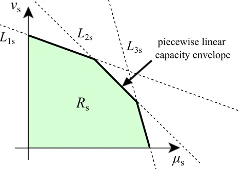
µs-νs plane, in order to avoid redundancy. For example, in Figure 1, the decision-maker may choose any point in the region Rs enclosed by the linesL1s, L2s, L3s and the coordinate axes, and this corresponds to a pair of service rates (µs, νs) to be used during interval s.
L
1sR
sμ
sν
spiecewise linear capacity envelope
L
2s [image:6.612.189.423.367.536.2]L
3sFigure 1: The piecewise linear capacity envelope for selection ofµs andνsat the beginning of time interval
s. For eachj∈ {1,2,3}, the lineLjs has equationγjsµs+νs ≤θjs.
In fact, it can be assumed that the decision-maker always chooses a point on the upper boundary of
Rs, since the objectives that we consider in this paper imply that one should always choose the largest possible value ofνs for a given value ofµs (this can be shown using a simple sample path argument, which we have omitted here). It follows that the decision-maker only needs to choose one value (µs) at each time interval, withνs then being given via the dominant linear constraint.
which depends on aircraft separation requirements, approach speeds, runway occupancy times and other data. Recently, Jacquillat and Odoni [30] recommended interpreting each point on the piecewise linear envelope as a pair ofaverage service rates for arrivals and departures (taking into account the uncertainty involved in actual take-off and landing times) and referred to the envelope as an operational throughput envelope (OTE). This interpretation makes more sense in the context of our paper, since we are treating eachµs(orνs) as anexpected number of service completions per unit time for classA(orD) during interval
s, rather than an upper bound. In reality, the exact shape of an OTE is interval-dependent and cannot be predicted with certainty for future time intervals, since it depends on weather conditions and also the mix and sequencing of different types of aircraft entering the queues for the runways. However, airports invariably have sophisticated meteorological equipment available for making weather forecasts and the mixture of air (or ground) traffic at an arbitrary point in time is heavily dependent on the predetermined schedule for arrivals (or departures), so it is reasonable to suppose that the OTEs for time intervals in the not-too-distant future can be predicted with a high degree of confidence.
The system evolves as a pair of independent, first-come-first-served queues of type M(t)/Ek(t)/1 or
P SRA/Ek(t)/1, depending on the nature of the arrivals processes. We assume that the service rates selected at the beginning of any time interval are chosen with knowledge of the latest observed numbers of customers waiting in both queues, the random distribution of future arrival times and the service rate constraints for future intervals. In the PSRA case, the history of previous customer arrivals affects future random arrival times and we assume that this historical information is also known.
2.2 The objective function
We assume that the objective of the decision-maker is to find an admissible dynamic policy π for choosing the service ratesµ1, µ2, ..., µS which minimizes
S X
s=1
EπαXs2+Ys2|x0, y0
+β
S X
s=2
[kτ(µs−µs−1)]2, (1)
where Xs and Ys are the respective numbers of Erlang service phases for customers of classes A and D remaining to be processed at the end of intervals,x0 and y0 are the initial values for these phase counts,
k is the number of Erlang service phases per customer (as stated in Section 2.1),τ =t1−t0 is the length of each time interval, and α >0 and β ≥0 are constants. The quantity [kτ(µs−µs−1)]2 (which may be
interpreted as the squared difference in the expected number of service phase completions between intervals
s and s−1 if the server remains constantly in use) represents the switching cost of changing the service rate (for class A) from µs−1 toµs. Thus, the decision-maker aims to minimize the sum of two terms: a weighted, aggregated measure of the congestion in the system over all time intervals, and a penalty which increases with the frequency and severity of changes made to the service rates.
to set-up costs, etc. However, in some applications the inclusion of a switching cost may be unnecessary and throughout this paper we make special reference to the case β= 0.
Weighted second moments of queue lengths have previously been used in [30] as a performance measure, although in our case the formulation is slightly different becauseXsandYsrepresent the numbers of service phases (not customers) present after stime intervals. Throughout this paper, we refer to the number of phases present as thephase count. The factorα allows for the possibility of classAcustomers being more expensive to keep waiting than classD customers, or vice versa.
The use of weighted second moments in our objective function can be justified in various different ways. Due to the nature of the Erlang service process, ifn≥1 customers are present in one of the queues (including the customer being served), then the phase count r satisfies (n−1)k+ 1 ≤ r ≤ nk, where k
is the Erlang parameter. As explained in [30], the total of the expected delays for n= dr/ke customers of the same class present in the system (where d·e denotes the ceiling function) is indeed of order n2 and therefore also of order r2. Furthermore, taking into account the second moments ofXs and Ys assists us in finding policies which will restrict the tails of their distributions, so that the system performs better with respect to measures such as the proportion of “on-time” service completions (as discussed in the introduction). In real-world applications, of course, practitioners are likely to be interested in meaningful performance measures rather than convoluted objective functions, and therefore it is desirable to show that a policy which performs well with respect to the objective 1 also achieves strong results with respect to other criteria. Later in this paper, we will examine the performance of our heuristics with respect to an alternative performance measure (expected waiting times) using numerical experiments.
2.3 MDP formulation
The problem that we are considering can be modelled as a Markov decision process (MDP) [39, 41] with a finite time horizon in which we aim to minimize expected total cost. Below, we describe the state space, action space, transition probabilities and single-stage cost function for the MDP.
• The state spaceof the MDP, which we will denote byX, consists of vectors of the form
x=
(x, y,µ¯)∈Z2
≥0×R≥0, [Poisson case], (x, y, z, w,µ¯)∈Z≥40×R≥0, [PSRA case],
(2)
wherex and y are the latest observed phase counts for the respective customer classes and ¯µ is the service rate for classA used in the previous time interval (this can be given a dummy value for the first interval). In the PSRA case, the extra state variables z and w are the numbers of class A and D customers respectively whose arrivals are ‘imminent’, in the sense that they have not yet arrived despite their earliest possible arrival times having passed (in other words, their exponential ‘clocks’ have already started running). Note that the memoryless property of the ξi variables implies that we do not need to know specifically which of the pre-scheduled arrivals have not yet occurred; we only require the number of imminent arrivals for each customer type. The inclusion of ¯µ as a state variable implies that the state space is uncountable, unless we are considering the special caseβ = 0 in which case ¯µ may be omitted.
rates µs which satisfy the feasibility constraints described in Section 2.1 (based on the relevant OTE). Specifically, given a set of constraints of the form γjsµs+νs ≤ θjs in interval s, we require 0≤ µs ≤minj{θjs/γjs}. As explained in Section 2.1, we can then assume that the complementary service rateνs is given by θjs−γjsµs.
• Transition probabilities for our MDP are governed by the underlying nonstationary queueing dynamics. For example, in the case of Poisson arrivals, these probabilities are based on the Chapman-Kolmogorov equations for M(t)/Ek(t)/1 queues (see, for example, [22]). We have included a full description of these equations in Appendix A.1.
• The one-stage cost functionis related to the objective function (1) and can be defined as
fs(x, µs) :=E[αXs2+Ys2|x, µs] +β(kτ)2(µs−µ¯)2. (3)
• The Bellman optimality equationcan be written, forx∈ X, as
Vs(x) = min µs∈Θs
n
fs(x, µs) +E[Vs+1(Xs)|x, µs] o
(s∈ {1,2, ..., S}), (4)
where Θsis the feasible set of service rates for intervals,Xsis the random state at the end of interval
s and we set VS+1(x) := 0 for all states x since our objective function (1) does not include costs incurred beyond the end of slotS. The functionsV1, V2, ..., VS are referred to asvalue functions. We also useV(x) :=V1(x) to denote the optimal expected total cost starting from state x.
The inclusion of phase counts in our cost and objective functions makes sense from an optimization perspective, since we should be able to obtain stronger-performing policies by considering the fine-grain state of the system. However, we note that the phase counts are a mathematical construct and in physical applications would not be observable by a decision-maker. Instead, decisions would be taken in response to the numbers of customers in the queues. In this paper, we take the approach of finding an optimal phase-dependent policy (allowing decisions to depend on the exact phase counts), and then aggregating this to obtain acustomer-dependent policy which chooses the same decision at any two states (x, y, z, w,µ¯) and (ˆx, y, z, w,µ¯) such that x,xˆ∈ {(n−1)k+ 1, ..., nk} for some n∈N. Various methods of aggregation are possible, but in this paper we adopt a simple averaging method which works as follows: given that n
andmcustomers are observed in theAandDqueues respectively and ¯µis the service rate for the previous time interval, let the service rate chosen for classAbe the mean of the service rates specified by the phase-dependent policy at thek2 states (x, y, z, w,µ¯) satisfying both (n−1)k≤x≤nk and (m−1)k≤y≤mk. Our simulation results in Section 6 incorporate this aggregation method.
3
The “Servers Always Busy” (SAB) approximation
As discussed in the introduction, we aim to make progress by restricting attention to an interval of time [0, T] during which there is a high probability of both queues remaining non-empty. Initially, we will consider the first of the two cases for arrival times described in Section 2, in which customers arrive via nonhomogeneous Poisson processes. For class A, we use λ(t), µ(t) andX(t) to denote (respectively) the arrival rate, the service rate and the number of phases remaining to be completed (i.e. the phase count) at timet, wheret∈[0, T] is a continuous time variable. For classD, the corresponding functions are denoted by η(t),ν(t) and Y(t). Let us also define two random variables ˆX(t) and ˆY(t) by
ˆ
X(t) =x0+kA(t)−B(t), Yˆ(t) =y0+kD(t)−C(t) ∀t∈[0, T], (5)
where x0 =X(0) and y0 =Y(0) are the initial phase counts and A(t), B(t), D(t) andC(t) are mutually independent Poisson random variables:
A(t)∼Po
Z t
0
λ(u)du
, B(t)∼Po
k
Z t
0
µ(u)du
,
D(t)∼Po
Z t
0
η(u)du
, C(t)∼Po
k
Z t
0
ν(u)du
. (6)
Note that B(t) and C(t) are phased-based measures (service phase completion counts), but A(t) and
D(t) are customer-based measures (customer arrival counts). If the servers are always busy during [0, T] then the customer arrival and service phase completion processes for the individual queues are indeed independent Poisson processes and we have ˆX(t) ≡ X(t) and ˆY(t) ≡ Y(t), i.e. Xˆ(t) and ˆY(t) mirror the physical state of the system. If the servers are almost always busy during [0, T] then we can expect
ˆ
X(t) and ˆY(t) to provide good approximations for X(t) and Y(t). In such cases, we can approximate the probability distributions at t ∈ [0, T] by exploiting their relations to the random variables in (6). If t is sufficiently large, we can make this process more practical computationally by claiming that, by the central limit theorem, ˆX(t) and ˆY(t) are approximately normally distributed with means and variances given as follows:
ˆ
X(t)∼Nx0+ Z t
0
k(λ(u)−µ(u))du,
Z t
0
(k2λ(u) +kµ(u))du,
ˆ
Y(t)∼N
y0+ Z t
0
k(η(u)−ν(u))du,
Z t
0
(k2η(u) +kν(u))du
. (7)
On the other hand, suppose we are considering the second case (PSRA) described in Section 2, whereby customer arrival times are randomly displaced from their pre-scheduled times. For simplicity we will describe the situation only for the first queue (with stateX(t)); the situation for theY(t) queue is obviously analogous. Let ωi denote the scheduled arrival time of the ith customer, so that ωi−ξ¯A is their earliest
possible time of arrival. We consider a random variable
ˆ
wherex0=X(0) and B(t)∼Po
kRt
0µ(u)du
(as before), but this time
A(t) =H1(t) +H2(t) +...+Hm(t) (9)
with m= max{i:ωi−ξ¯A < t}. Here, Hi(t) is a Bernoulli random variable equal to 1 if theith customer arrives before timet and 0 otherwise. Hence,
E[A(t)] = m X
i=1
pi(t), Var[A(t)] = m X
i=1
pi(t)(1−pi(t)),
where
pi(t) = 1−exp
−t−ωi+ ¯ξA ¯
ξA
.
If approximations are required for state probabilities, then (as in the Poisson case) we can make use of the central limit theorem for sufficiently largetand write
P( ˆX(t)≤n)≈Φ
n+ 0.5−E[ ˆX(t)] q
Var[ ˆX(t)]
(10)
forn∈N, withE[ ˆX(t)] and Var[ ˆX(t)] derived from (8) (this holds since the variablesHi(t) are independent of each other, albeit not identically distributed). However, the ADP methods that we develop later in this paper do not actually require approximations for state probabilities.
Taking into account the importance of being able to apply our methods to real-world scenarios, we tested the quality of the SAB approximation using data obtained from John F. Kennedy International Airport in New York. Our experiment included time-dependent Poisson demand rates for arrivals and departures which were constructed using a particular flight schedule, and two different sets of capacity constraints (OTEs) based on alternative weather scenarios. Based on these capacity constraints, a naive ‘greedy’ heuristic was used to select the time-varying service rates and the quality of the SAB approximation was then tested by comparing its estimates for the objective function (1) with ‘exact’ values derived using Chapman-Kolmogorov equations. A full description of our experimental procedure and results can be found in Appendix A.2, and we also summarize the results here:
• We found that, throughout a period of time beginning at roughly 4:30PM and ending at roughly 10:00PM on the day of operations that we considered, the arrivals queue and the departures queue both had idleness probabilities smaller than 0.05 in the ‘good weather’ case. In the ‘poor weather’ case, these probabilities were consistently smaller than 0.03.
• The error incurred by using the SAB approximation to estimate the objective function (1) over a period of 22 consecutive 15-minute time intervals, beginning at 4:30PM and ending at 10:00PM, was only 0.26% in the good weather case, and 0.02% in the poor weather case.
• In the poor weather case, it was possible to consider a longer time period beginning at 3:15PM and ending at 11:15PM without incurring a SAB approximation error greater than 0.5%.
poten-tial to improve the quality of decision-making at JFK Airport during a schedule-dependent ‘busy’ period of the day (e.g. 4:30PM to 10:00PM) by making use of the SAB approximation.
4
A surrogate optimization problem
As discussed earlier, the MDP formulated in Section 2.3 cannot be solved using conventional dynamic programming (DP) methods. We therefore aim to develop heuristic policies which are based on the simplified queueing dynamics discussed in Section 3.
In this section we introduce a surrogate optimization problem which closely resembles the problem formulated in Section 2, especially in cases where customer demand is consistently high in relation to service capacity. As discussed in the introduction, we intend to utilize this surrogate problem by (i) characterizing myopic policies and investigating the conditions under which these perform well; (ii) investigating the nature of optimal policies by finding quadratic approximations for the value functions in terms of the state variables; (iii) developing heuristic methods for theoriginal (not the surrogate) optimization problem based on the properties of these myopic policies and quadratic approximating functions.
Please note that throughout this section we will make repeated use of the variables x, y, z,w and ¯µ
(as in (2)) to represent a generic observed state at the beginning of an arbitrary time intervals, without including an explicits-dependence on these variables.
The surrogate problem differs from the problem formulated in Section 2 in the following ways:
1. For each s∈ {1,2, ..., S}, we remove the constraint µs ∈Θs and allow the service rate µs (for class
A) to take any positive or negative real value, with the corresponding service rate νs (for class D) then being given by the dominant linear constraint. Specifically, given a set of Js linear constraints
{γjsµs+νs≤θjs}Jj=1s , the feasible region for (µs, νs) is now
{(µs, νs)∈R2:νjs≤θjs−γjsµs ∀j∈ {1,2, ..., Js}}
and is therefore an infinite region given by the intersection of closed half-planes.
2. Following the selection of (µs, νs)∈R2 in time intervals, the random phase countsXsand Ys at the end of interval sare given by
Xs=x+kAs−sgn(µs)Bs, Ys =y+kDs−sgn(νs)Cs, (11)
where sgn(·) denotes the signum function,x and y are the phase counts at the beginning of interval
s, and As, Bs, Cs and Ds are mutually independent, discrete random variables. In particular, As and Ds (which represent the numbers of customer arrivals during interval s) obey the same laws as in the original problem and these depend on which case we are considering for the demand processes (either Poisson or PSRA). We defineBs andCs as follows:
Bs∼Po(kτ|µs|), Cs∼Po(kτ|νs|).
We will denote the one-step cost function in the surrogate problem by
gs(x, µs) :=E[αXs2+Ys2|x, µs] +β(kτ)2(µs−µ¯)2, (12)
so that it essentially has the same definition as fs(x, µs) (in the original problem) except that the expec-tation is with respect to the dynamics of the surrogate problem. The objective in the surrogate problem is to find a dynamic policy π for choosing µ1, µ2, ..., µS ∈Rwhich minimizes
U(x) :=Eπ " S
X
s=1
gs(xs, µs)
x0 =x #
. (13)
Throughout Sections 4 and 5 we will assume that the time interval durationτ is equal to one. This is without loss of generality, since the demand rates and service rates can always be re-scaled appropriately. We should also note that the objective function (13) implies that, as in the original problem, the service rates (µs, νs) should always be chosen on the upper boundary of the feasible region. Therefore the notation in (12) makes sense, since the complementary service rate νs is given as a deterministic function of µs via the dominant linear constraint.
By assuming that the random variables in (11) are independent, we implicitly relax the constraints on the phase counts Xs and Ys by allowing them to take negative values. Effectively, we are considering a mathematical abstraction of our original problem in which servers remain busy at all times and can cause phase counts to either increase or decrease (depending on the signs of the service rates). Naturally, this abstraction makes it easier to perform analyses since we are approximating the queueing dynamics of the original system using independent random variables. At the same time, our analyses should provide useful insights into the nature of optimal policies during busy periods in which phase counts are likely to remain positive. In addition, given that (µs, νs) must be located on the upper boundary of the feasible region, a negative value for eitherµsorνs implies that|µs−νs|is relatively large, i.e. it implies imbalanced service rates. We can argue that imbalanced service rates are unlikely to be chosen by the decision-maker under certain plausible cases for the parameters of our problem, as described below:
(i) The nature of the objective function (1) implies that, under an optimal policy, the decision-maker should try to maintain an appropriate balance between the phase counts Xs and Ys. Hence, imbal-anced service rates will usually not be advantageous unless there is a significant imbalance between demand rates and/or service rate constraints for classesAand D.
(ii) The incorporation of non-zero switching costs (i.e. setting β > 0) will tend to deter the decision-maker from making drastic changes to the service rates from one time interval to the next, thereby reducing the likelihood of a negative service rate being chosen.
(iii) If the variances of As and Ds are relatively small (which may happen if we are considering pre-scheduled arrival times, for example) then the variances of Xs and Ys will also be small, further reducing the likelihood of the decision-maker needing to select imbalanced service rates.
classes A and D with respect to time-varying demand rates and service rate constraints; (iii) non-zero switching costs; (iv) small variances for customer arrival times. Of course, these conditions may not necessarily be satisfied in real-world applications, but if theyare satisfied then this should imply a stronger performance for the heuristics that we derive in Section 5. Numerical experiments can be used to illustrate the effects of varying demand rates, service rate constraints etc. (see Section 6).
In searching for an optimal policy which minimizes (13), a useful starting point is to find a myopic policy which operates by minimizing the expected single-step cost gs(x, µs) at each time interval s. In Section 4.1 we provide characterizations for myopic policies, and in Section 4.2 we examine the nature of optimal policies for our surrogate problem.
4.1 Myopic policies
Our assumptions regarding the set of linear constraints {γjsµs+νs ≤θjs}Jj=1s are the same as in the original version of the problem. Specifically, we assume thatγ1s< γ2s< ... < γJs,sand that the intersection point between any pair of consecutive constraints γjsµs+νs =θjs and γj+1,sµs+νs = θj+1,s, which we will denote by σjs, lies within [0, θJs,s/γJs,s] (otherwise there would be at least one redundant constraint in the original problem). Using this notation, we can state that
νs =
θ1s−γ1sµs, ifµs≤σ1s,
θ2s−γ2sµs, ifσ1s≤µs≤σ2s, ..
. ...
θJs−1,s−γJs−1,sµs, ifσJs−2,s ≤µs≤σJs−1,s,
θJs,s−γJs,sµs, ifµs≥σJs−1,s.
(14)
We are seeking to find a myopic decision which minimizes the function gs(x, µs) defined in (12). For ease of notation, let the intervals (−∞, σ1s),(σ1s, σ2s), ...,(σJs−2,s, σJs−1,s),(σJs−1,s,∞) be denoted by Ω1s,Ω2s, ...,ΩJs,s respectively. On each of the intervals Ωjs, we can check to see if gs(x, µs) attains a local minimum. First, evaluating the means and variances of Xs and Ys, we have
E[Xs|x, µs] =x+k(E[As|x]−µs), E[Ys|x, µs] =y+k(E[Ds|x]−(θs−γsµs)), (15) Var[Xs|x, µs] =k(kVar[As|x] +|µs|), Var[Ys|x, µs] =k(kVar[Ds|x] +|θs−γsµs|). (16)
Hence, evaluating the second moment of Xs, we have
E[Xs2|x, µs] = (terms independent of µs) +k2µ2s−kµs(2x+ 2kE[As|x]) +k|µs|, (17)
whereE[As|x] depends on the nature of the demand process for classA; for example, in the case of Poisson arrivals with demand rateλ(t),As is independent of xand we haveE[As] =
Rts
ts−1λ(u)du. Similarly, given
an interval on whichνs =θjs−γjsµs, we have
E[Ys2|x, µs] =(terms independent ofµs) +k2(θjs−γjsµs)2−k(θjs−γjsµs) (2y+ 2kE[Ds|x])
It follows from (17) and (18) that gs(x, µs) is a continuous, piecewise quadratic function of µs. The boundaries between the quadratic pieces include the verticesσjs(forj= 1,2, ..., Js) and also the end-points of the interval [0, θJs,s/γJs,s] at which the service rates change sign. On each quadratic piece, we can check to see if a local minimum is attained. The expressions for these local minima depend on the dominant linear constraints in the regions in which they are found, and also on the signs ofµsandνsin these regions. For example, if a local minimum is attained at some point µs ∈(0, θJs,s/γJs,s) in which thej
th constraint
is dominant, then the expression for this local minimum is
2αx−2γjsy+ 2k(αE[As|x]−γjsE[Ds|x] +γjsθjs+βµ¯) +γjs−α
2k(α+γ2js+β) . (19)
Other possible cases are discussed in Appendix A.3. To simplify the search for a global minimizer of
gs(x, µs) we provide the following result, which is proved in Appendix A.3.
Proposition 4.1. The function gs(x, µs) is continuous and unimodal with respect to µs ∈R. Hence, for each state x∈ X, there exists µMYPs (x) ∈ R such that gs(x, µs) is strictly decreasing for µs < µMYPs (x), and strictly increasing for µs> µMYPs (x).
From Proposition 4.1 it follows that the service rateµMYPs (x) which minimizes gs(x, µs) can be found using a simple procedure which requires a negligible amount of computation time. For eachj∈ {1,2, ..., Js}, letµMYPjs (x) denote the unique local minimum ofgs(x, µs) if we assume that the relationshipγjsµs+νs =θjs applies for all µs ∈ R (it is proved in Appendix A.3 that this value µMYPjs (x) exists, although in certain cases it may be a non-differentiable point). The resulting value µMYPjs (x) may or may not be contained in Ωjs. If µMYPjs (x) ∈ Ωjs for some j ∈ {1,2, ..., Js}, then Proposition 4.1 implies that µMYPjs (x) is also the global optimizer µMYPs (x). On the other hand, ifµMYPjs (x) ∈/ Ωjs for all j ∈ {1,2, ..., Js}, then the global minimum is one of the vertices {σ1s, ..., σJs,s}, which we will denote byσ
∗
s. With this notation, we can conclude that the myopic service rate is given by
µMYPs (x) =
µMYPjs (x), if∃j ∈ {1,2, ..., Js}such that µMYPjs (x)∈Ωjs,
σs∗, otherwise.
(20)
4.2 Optimal policies
Although the surrogate problem that we are considering enables myopic service rates to be calculated quite easily, finding a policyπwhich minimizes the objective function (13) remains a challenging problem. Our approach in this section is to look for a simple approximation to U(x) (specifically, a parametric function of the system statex) and use this approximation to develop a heuristic approach.
4.2.1 A single, time-varying linear constraint
Let us consider the case where a single linear constraint of the form γsµs+νs ≤ θs applies at time intervals∈ {1,2, ..., S}. The Bellman equation for the surrogate problem can be written
Us(x) = min µs∈R
n
gs(x, µs) +E[Us+1(Xs)|x, µs] o
(s∈ {1,2, ..., S}), (21)
where U1, ..., US are finite-stage value functions and US+1(x) := 0 for all x ∈ X. We aim to find the minimizing value ofµs in (21), assuming that the relationships νs=θs−γsµs hold for intervalss.
Let us begin by consideringUS(x), the optimal return under state xwith only one interval remaining until the end of the horizon. Naturally, a myopic choice of service rate is optimal at this interval. Although we are considering a single linear constraint, the cost function gS(x, µS) still exhibits piecewise quadratic behavior due to the nature of the variances in (16) as the service rates change sign (this is explained further in Appendix A.3). Ideally, we would like to express US(x) as a simple quadratic function of the state variables, but the piecewise behavior of gS(x, µS) prevents this. However, we can derive a lower bound forUS(x) by omitting the modulus signs in (16) and writing
gS(x, µS)≥α
k2µ2S−kµS(2x+ 2kE[AS|x]−1)
+k2(θS−γSµS)2−k(θS−γSµS) (2y+ 2kE[DS|x]−1)
+βk2(µS−µ¯)2+ (terms independent of µS). (22)
Equality holds in (22) if and only if µS and νS = θS−γSµS are both non-negative, which (as we have argued earlier) is likely to be the case for many statesx∈ X under plausible modelling assumptions. Let us consider the random variables AS and DS. In the case of Poisson arrivals, these are actually independent of the system statex. In the case of pre-scheduled arrivals, AS and DS depend on x, but it is useful to note that E[AS|x] and E[DS|x] are linear in their dependencies on the state variablesz and w (which represent the numbers of ‘imminent arrivals’) respectively. Indeed, this linearity property holds for arbitrary s∈ {1,2, ..., S}, since we can write
E[As|x] =zp0+ S−s X
j=1
Ls+jpj, Var[As|x] =zp0(1−p0) + S−s X
j=1
Ls+jpj(1−pj), (23)
E[Ds|x] =wq0+ S−s X
j=1
Ms+jqj, Var[Ds|x] =wq0(1−q0) + S−s X
j=1
Ms+jqj(1−qj), (24)
whereLj (resp. Mj) is the number of customers of class A(resp. D) scheduled to arrive at the beginning of intervalj, andpj (resp. qj) is the probability that a customer of class A(resp. D) scheduled to arrive at the beginning of interval s+j arrives during interval s. (Note: this notation makes sense whenj = 0 since, due to the memoryless property, we can treat all customers who have not yet arrived by interval
Minimizing the right-hand side of (22) overµS ∈Ryields a local minimum at
µS =
2αx−2γSy+ 2k(αE[AS|x]−γSE[DS|x] +γSθS+βµ¯) +γS−α 2k(α+γ2
S+β)
, (25)
and with this value of µS, the right-hand side of (22) can be expressed as
USLB(x) :=xTPSx+qTSx+rS, (26)
where PS is a matrix of order n×n (where n is the number of state variables), qS ∈ Rn and rS ∈ R. Importantly,PS,qS and rS do not have any dependence onxorµs. We can infer from (26) that USLB(x) is a quadratic function of the state variables. Note that the number of state variablesn can be 2, 3, 4 or 5, depending on the type of arrivals distribution and the value of β. For example, in the case of Poisson arrivals withβ = 0, we havex= (x, y)∈Z2 and it can be shown that
PS =
α α+γS2
"
γS2 γS
γS 1 #
, qS= 1
α+γS2
α(α−γS) + 2kαγS(γSE[AS|x] +E[DS|x]−θS)
γS(γS−α) + 2kα(γSE[AS|x] +E[DS|x]−θS)
.
(We have omitted the expression forrS because it is too long.) Evidently,USLB(x) is a lower bound for
US(x) since the latter is obtained by minimizinggS(x, µS), whereas the former is obtained by minimizing an expression which is bounded above by gS(x, µS). Let us proceed by obtaining lower bounds for Us(x) for each s∈ {1,2, ..., S−1}. We propose the following lemma.
Lemma 4.2. Suppose that, for a particular interval s ∈ {1,2, ..., S −1}, there exists a function UsLB+1 : X →Rsuch that
UsLB+1(x) =xTPs+1x+qTs+1x+rs+1 ≤Us+1(x) ∀x∈ X, (27) where Ps+1 is a real-valued matrix of order n×n, qs+1 ∈ Rn, rs+1 ∈ R and n is the number of state variables. Let UsLB:X →Rbe defined by
UsLB(x) = min µs∈R
n
gs(x, µs) +ψs(µs) +E[UsLB+1(Xs)|x, µs] o
, (28)
where
ψs(µs) =
2k(α+ ˜As+1)µs, if µs<0,
2k(1 + ˜Bs+1)(θs−γsµs), if µs> θs/γs,
0, otherwise,
(29)
andA˜s+1 andB˜s+1 are the coefficients of x2 andy2 respectively in the expression for UsLB+1(x). Then there exists a real-valued n×nmatrix Ps, a vector qs∈Rn and a constant rs∈Rsuch that
UsLB(x) =xTPsx+qTsx+rs ≤Us(x) ∀x∈ X. (30)
eitherµsorνs=θs−γsµs is negative thenψs(µs) takes an artificial non-zero value in order to ensure that a quadratic representation of UsLB(x) is still possible.
By using the result of Lemma 4.2 iteratively, we can find suitable values Ps,qs and rs satisfying (30) for each s∈ {1,2, ..., S}. We can then write
UsLB(x)≤Us(x)
for any statex∈ X ands∈ {1,2, ..., S}. Generally it is not worthwhile to write expressions forPs,qs and
rs in terms of the system parameters, since these expressions are too convoluted. However, an interesting special case occurs whenβ = 0 and the OTE is the same for each time interval, so that γs=γ and θs =θ for each s∈ {1,2, ..., S}. This is the subject of the next subsection.
4.2.2 A single, fixed linear constraint with β= 0
The following lemma states what may be proved in this special case.
Lemma 4.3. Suppose β = 0and we have a single linear constraint γµs+νs≤θ for each s∈ {1,2, ..., S} (where γ, θ >0). Then, for a particular slots∈ {1,2, ..., S}:
(a) In the case of Poisson arrivals, we have
UsLB(x) = ˜As(γx+y)2+ ˜Bs(γx+y) + ˜Cs(αx−γy) + ˜Ds ∀x∈ X, (31)
where A˜s, B˜s, C˜s and D˜s are constants which depend on the system parameters. In particular, the values of A˜s, B˜s and C˜s are given by
˜
As=
(S−s+ 1)α
α+γ2 , B˜s=
2kαPS
j=s(S−j+ 1)(γE[Aj] +E[Dj]−θ)
α+γ2 ,
˜
Cs =
α2−γ3+ (S−s+ 1)αγ(γ−1)
(α+γ2)2 . (32)
(b) In the case of pre-scheduled arrivals, we have
UsLB(x) = ˜As(γx+y)2+ ˜Cs(αx−γy) + ( ˜Fs+ ˜Gsz+ ˜Hsw)(γx+y)
+ ˜Jsz2+ ˜Ksw2+ ˜Lszw+ ˜Msz+ ˜Psw+ ˜Zs ∀x∈ X, (33)
where A˜s, C˜s, F˜s, G˜s, H˜s, J˜s, K˜s, L˜s, M˜s, P˜s and Z˜s are constants which depend on the system parameters. In particular, A˜s and C˜s have the same values as in (32).
Furthermore, the service rate µOPTs (x) which attains the minimum in (28) is
µOPTs (x) =
µMYPs (x) +δ, if s < S,
µMYPs (x), if s=S,
where
δ = γ(1−γ) ˜As+1+ (α+γ 2) ˜C
s+1 2k(α+γ2) =
α2−γ3
2k(α+γ2)2 (35)
and µMYP
s (x) is the myopic service rate:
µMYPs (x) = 2αx−2γy+γ−α+ 2k(αE[As|x]−γE[Ds|x] +γθ)
2k(α+γ2) . (36)
The proof of Lemma 4.3 can be found in Appendix A.6. If we consider a problem in which the cost functiongs(xs, µs) is replaced bygs(xs, µs) +ψs(µs), then (35) provides us with a simple condition for the optimality of a myopic policy. We state this below as a corollary.
Corollary 4.4. Consider a decision problem in which we aim to minimize
ULB(x) =Eπ " S
X
s=1
(gs(xs, µs) +ψs(µs))
x0 =x #
, (37)
whereπis a policy for choosing the service ratesµ1, µ2, ..., µS∈R. We assume a single constraintγµs+νs≤
θ applies for all s∈ {1,2, ..., S} andβ = 0. Then a myopic policy is optimal if and only if α2 =γ3. Proof. The value functions for the problem described in the corollary are UsLB(x), defined recursively via (28). By Lemma 4.3, we see that an optimal policy (with respect to UsLB(x)) differs from a myopic policy by adding a constant term (α2−γ3)/(2k(α+γ2)2) to the myopic service rate, and hence the myopic and optimal policies coincide if and only ifα2=γ3.
It is important to note that the relationshipα2=γ3 holds if α=γ = 1, in which case the two classes of customer are equivalent with respect to both congestion charges and resource consumption rates. This might apply to many types of application in which there is no obvious reason to treat one class of customer differently from another. The fixed service rate adjustmentδ increases withα but decreases withγ, which is logical given the physical interpretations of these parameters.
Although Corollary 4.4 is related toULB(x) rather than our original value functionU(x), the differences
U(x)−ULB(x) should be relatively small if (i) the optimal policy for the surrogate problem rarely chooses negative service rates, and (ii) phase counts for the surrogate problem rarely become negative. At the beginning of Section 4 we suggested conditions under which these effects should be observed.
In Appendix A.5 we have provided a numerical example in which customers of classesA andD arrive according to Poisson processes with complementary sinusoidal demand rates. Our example considers the caseα=γ = 1 and uses Lemma 4.3 to compute the exact values of UsLB(x) fors∈ {1,2, ..., S}. Estimated upper bounds forU(x) are then obtained by simulating the performance of a myopic policy in the surrogate problem. Since the optimal value U(x) is (by definition) bounded above by the value UMYP(x) obtained under a myopic policy, the estimates ofUMYP(x)−ULB(x) obtained via simulation can be interpreted as estimated upper bounds forU(x)−ULB(x). Our results indicate that
• However, even in cases where total demand consistently exceeds capacity by as much as 100%,
UMYP(x)−ULB(x) is generally smaller than 0.25%.
We also repeated our experiments with different values ofα andγ, with similar results (please refer to Appendix A.5 for full details). The second of the bulleted points above is especially relevant in the context of this paper, since in problems where demand greatly exceeds capacity, we can expect the dynamics of our surrogate problem to closely resemble those of the original problem. We therefore have some evidence to suggest that, in the case of a single, fixed linear constraint withβ = 0, myopic policies are very close to optimal in the surrogate problem - and this should also apply to the original problem if demand rates are sufficiently high. Our numerical results in Section 6 will demonstrate the effects of time-varying service rate constraints and positiveβ values on the performances of myopic policies.
We will provide one further result here which concerns a ‘deterministic fluid flow analogue’ of our original optimization problem, in which queueing dynamics are deterministic and the workloads in the two queues are represented as continuous variables. Although this fluid flow model represents a significant departure from our original stochastic optimization problem, it does yield a condition for equivalence between the fluid flow analogues of U(x) and V(x) which may offer a useful practical guide for decision-making in the stochastic problem. Consider a variant of the problem formulated in Section 2 in which the state space is
R2≥0 and the phase counts at time t∈[ts−1, ts) during intervals∈ {1,2, ..., S} are
X(t) =x+k
Z t
ts−1
(λ(u)−I(X(u)>0)µs)du, Y(t) =y+k Z t
ts−1
(η(u)−I(Y(u)>0)νs)du,
where (x, y) is the state at the beginning of intervals,I(·) denotes the indicator function,λ(t) andη(t) are continuous flow rates andµsandνsare the chosen service rates for intervals, which are both non-negative and satisfyγµs+νs=θ. The phase counts at the end of interval sare Xs =X(ts) and Ys=Y(ts). The value function for this problem will be denoted by VFF(x), where
VFF(x) = min π
S X
s=1
αXs2+Ys2|x, π
and π is a decision-making policy which, in this deterministic setting, is simply a vector of service rates. In the ‘surrogate’ version of our fluid flow problem, we do not enforce non-negativity for either the service rates or the phase counts and we replace the definitions of X(t) and Y(t) above by
X(t) =x+k
Z t
ts−1
(λ(u)−µs)du, Y(t) =y+k Z t
ts−1
(η(u)−νs)du,
withUFF(x) used instead ofVFF(x) to represent the corresponding value function.
Proposition 4.5. In the deterministic fluid flow problem:
(a) The finite-stage value functions U1FF, ..., USFF satisfying the Bellman equations
UsFF(x) = min µs∈R
αXs2+Ys2+UsFF+1(Xs)|x, µs
(with USFF+1(x) := 0 for allx∈ X) are given by
UsFF(x) = ˜As(γx+y)2+ ˜Bs(γx+y) + ˜Ds ∀x∈ X, s∈ {1,2, ..., S},
where A˜s and B˜s have the same definitions as in (32) and D˜s is constant. For each interval s ∈
{1,2, ..., S}, the myopic and optimal service rates for the surrogate problem are given by
µOPTs (x) =µMYPs (x) = αx
−γy+kRts
ts−1(αλ(u)−γη(u))du+kγθ
k(α+γ2) . (39)
(b) Suppose the system is initialized in a state x= (x0, y0) which satisfies
0≤ αx0−γy0+α
Rt1
t0 λ(u)du−γ
Rt1
t0 η(u)du+γθ
α+γ2 ≤
θ
γ, (40)
and also suppose that
0≤ α
Rts
ts−1λ(u)du−γ
Rts
ts−1η(u)du+γθ
α+γ2 ≤
θ
γ (41)
for each s∈ {2, ..., S}. Let n0 = min{x0, y0}. Then
lim n0→∞
|UFF(x)−VFF(x)|= 0
and the service rates in (39) are optimal in both versions of the fluid flow problem.
Proposition 4.5, which is proved in Appendix A.7, provides us with conditions involving the demand rates and capacity envelope parameters which ensure that the simple myopic policy represented by (39) is also an optimal policy for both the surrogate problem and the original problem. Although the result concerns a modified version of the problem with deterministic fluid flow dynamics, the conditions (40) and (41) (or similar conditions adapted to the case of pre-scheduled arrivals) might also imply a strong performance for the aforementioned policy in the original stochastic problem, especially if the variances for end-of-interval phase counts Xs and Ys are small.
4.2.3 Multiple linear constraints
We now discuss the case of multiple linear constraints. As before, letJs be the number of constraints in interval s, so that the jth constraint (for j ∈ {1,2, ..., Js}) has the form γjsµs +νs ≤ θjs. Also, let (ns, ns+1, ..., nS) be an (S −s+ 1)-tuple, such that ni ∈ {1,2, ..., Ji} for i ∈ {s, s+ 1, ..., S}. The tuple (ns, ns+1, ..., nS) represents a sequence of individual constraints ‘chosen’ from the constraint sets for intervals s, s+ 1, ..., S. Given a particular tuple (ns, ns+1, ..., nS) we can obtain a quadratic function
U(LBn
s,ns+1,...,nS)(x) such that
U(LBns,n
s+1,...,nS)(x)≤Us(x) ∀x∈ X
by assuming that the relationshipνi=θni,i−γni,iµi holds for allµi ∈Rin intervali∈ {s, s+ 1, ..., S} and then constructing the quadratic functionU(LBn
for each of the intervals i ∈ {s, s+ 1, ..., S}, we are drawing a straight line over the top of the OTE for intervaliand deriving a lower bound by supposing that the decision-maker is allowed to choose any point on this line. However, the lower bound ULB
(ns,ns+1,...,nS)(x) obtained in this way is unlikely to be very tight if there are many constraints, since the local minima found on the unbounded straight lines will rarely satisfy the constraints for the actual surrogate problem. A tighter lower bound is given by
UsMLB(x) := max (ns,ns+1,...,nS)
U(LBn
s,ns+1,...,nS)(x),
but this is a piecewise quadratic function of x which cannot be computed easily due to the large number of possible tuples (ns, ns+1, ..., nS) that one must consider as S−sincreases.
A computationally feasible algorithm would need to be based on a simple representation of UsLB(x), similar to the quadratic functions that we were able to obtain in the case of single linear constraints. In Section 5 we introduce a number of heuristic policies, two of which are based on the idea of approximating the value functionsVs(x) using quadratic functions of the state variables.
5
Design of heuristics
In this section we introduce 4 different heuristics. All of these are dynamic decision-making policies which choose a service rateµsfor class Ain response to an observed system statex∈ X at time intervals (with the service rate for class D,νs, being given by the OTE for interval s). We present the 4 heuristics in increasing order of the amount of computational effort required.
All of the heuristics that we develop in this section are based on optimal (or near-optimal) solutions to thesurrogate problem described in Section 4, in which negative service rates and phase counts are per-mitted. However, in Section 6 we test the heuristics by applying them to the original problem formulated in Section 2 (which does not permit negative service rates or phase counts).
1. Myopic policy (MYP)
Under this policy, we choose the service rateµMYPs (x) which minimizes the expected single-stage cost at the end of interval s in the surrogate problem. As discussed in Section 4.1, µMYPs (x) can be found by searching for a local minimum of the function gs(x, µs) in each of the intervals Ωjs (for j = 1,2, ..., Js), and choosing an appropriate boundary point if no local minimum is found.
When implementing this heuristic in the original problem, we will need to enforce non-negativity by choosing µs = 0 if the myopic service rate µMYPs (x) defined in (20) is negative, or µs = θJs,s/γJs,s if
µMYPs (x) is greater than θJs,s/γJs,s (in which case we need to avoid a negative νs value). Due to the unimodality of gs(x, µs) proved by Proposition 4.1, it follows that this ‘truncated’ version of the myopic policy does indeed minimize gs(x, µs) if the extra constraints µs, νs≥0 are enforced.
2. Approximate Policy Improvement (API)
minimizes the estimated two-step return
gs(x, µs) +gs+1 E[Xs|x, µs], µMYPs+1 (E[Xs|x, µs])
, (42)
whereE[Xs|x, µs] is the expected state at the end of intervalsgiven that we choose service rateµs. Effec-tively, we are relying upon a forecast of the next state in order to predict the service rateµMYPs+1 (E[Xs|x, µs]) chosen by the myopic policy at the beginning of interval s+ 1, rather than taking into account the full distribution of µMYPs+1 (Xs) as a function of the random phase counts Xs and Ys (which would require a prohibitive amount of computational effort). This is why we describe the heuristic asapproximate policy improvement. For the final time interval S, a myopic service rate can be chosen. We also use the same truncation method as in the myopic policy, so that µs, νs∈[0, θJs,s/γJs,s].
In principle, we could extend this idea and obtain an approximate m-step improvement policy by cal-culating the best service rate for intervals under the assumption that myopic service rates are chosen for intervalss+ 1, s+ 2, ..., s+m. This method would also rely upon predictions of the myopic service rates for future time intervals based on expected values of the phase counts. However, our experiments have shown that any benefit obtained by implementing m-step improvement as opposed to one-step improvement is usually very slight, and in some cases it actually performs worse - perhaps because the forecasts for future phase counts become less reliable as the ‘look-ahead distance’ increases.
3. Coefficient Averaging (CAV)
This heuristic is motivated by the discussion in Section 4.2.3 and is intended as a fairly naive but inex-pensive method of acquiring quadratic approximations for the value functions in a problem with multiple linear constraints. It uses backwards induction, starting from the final time interval S. For each of the linear constraints γjSµS+νS ≤θjS effective at interval S, we construct the function
UjSLB(x) := min µS∈R
n
gjS(x, µS) +ψjS(µS) o
,
where gjS(x, µS) is similar to the usual single-step expected cost gS(x, µS) except that it assumes the relationshipνS =θjS−γjSµS holds for all µS∈R, and ψjS(µS) is similar to the functionψS(µS) defined in (29) except thatγS andθS are replaced byγjSandθjS respectively. The analyses in Section 4.2.1 imply that, for each j∈ {1,2, ..., JS},UjSLB(x) is a quadratic function of x.
We then create a new functionUSCAV(x) by considering each of the variablesx2,y2,xyetc. individually and, for each variable, averaging the relevant coefficients which appear in the functions UjSLB(x). For example, if we are considering Poisson arrivals with β = 0, then (as shown in Section 4.2.1) the functions
ULB
jS (x) are linear combinations of the variables
x2, y2, xy, x, y.
We therefore form a new function USCAV(x) which is also a linear combination of the above vari-ables. The coefficient of x2 in USCAV(x) is the arithmetic mean of the coefficients of x2 in the functions
U1LBS(x), U2LBS(x), ..., UJLB
S,S(x), and similarly for the coefficients of y
functionUSCAV−1(x), we start by obtaining the functions Uj,SLB−1(x) defined by
Uj,SLB−1(x) = min µS−1∈R
n
gj,S−1(x, µS−1) +ψj,S−1(µS−1) +E[USCAV(XS−1)|x, µS−1]
o
.
As demonstrated by the analyses in Section 4.2.1, the functions Uj,SLB−1(x) are linear combinations of the same variables as the functionsUjSLB(x). We can therefore obtain a function USCAV−1(x) using the same coefficient-averaging procedure as that used for USCAV(x), and we repeat these steps to obtain functions
USCAV−2(x), USCAV−3(x), ..., U1CAV(x). The CAV heuristic chooses the service rate µCAVs (x) ∈ [0, θJs,s/γJs,s] which attains the minimum in the expression forUsCAV(x).
4. Least-squares Fitting (LSF)
This heuristic, like the previous one, is based on backwards induction and the use of a parametric function of the system state to approximate the value functions Vs(x). In this case we assume, a priori, that Vs(x) can be well-approximated by a quadratic function of the state variables and use least-squares fitting (after ‘sampling’ the values at a selection of states) to find suitable values of the coefficients that appear in this quadratic function. The steps are as follows:
1. Sets=S and ˆVS+1(x) = 0 for all statesx∈ X.
2. Select a certain number of system states in X either randomly or systematically (choosing a large number of states should yield a stronger performance at the expense of greater computation time). LetMs⊂ X denote the set of states chosen.
3. For eachx∈Ms, calculate the value
Ws(x) := min µs∈Θs
n
gs(x, µs) +E[ ˆVs+1(Xs)|x, µs] o
. (43)
4. Use least-squares regression to minimize
X
x∈Ms
Ws(x)−Qs(x) 2
(44)
where Qs(x) is quadratic in the state variables and the minimization is carried out with respect to the coefficients inQs(x). Let ˆVs(x) denote the function Qs(x) which minimizes (44).
5. Reduces by 1. Ifs≥1 return to step 2; otherwise, stop.
The LSF heuristic chooses the service rateµLSFs (x)∈Θs which attains the minimum in (43).
6
Numerical experiments
‘baseline’ decision-making policy which might be employed by a decision-maker in practice. In Section 6.1 we describe our baseline heuristic. The majority of our numerical results are presented in Section 6.2, and in Section 6.3 we investigate the effects of our heuristics on customer waiting times.
6.1 A naive baseline heuristic
The naive heuristic that we introduce here, which we will refer to as a “myopic demand ratio” (MDR) heuristic, is based on a measure of the demand placed on the server by customers of classAas a proportion of the total demand imposed by both customer classes over a single time interval. The heuristic works as follows: at the beginning of interval s∈ {1,2, ..., S}, the decision-maker observes the phase counts x and
y for classes Aand D respectively and also calculates the expected numbers of customers arriving during intervals,E[As|x] andE[Ds|x]. Taking into account that customers of classAare more expensive to hold in the queue by a factorα, the decision-maker calculates the ‘effective demand ratio’ as
α(x+kE[As|x])
y+kE[Ds|x]
. (45)
They then select the unique point (µs, νs) on the OTE for interval s which results in the ratio µs/νs being equal to the effective demand ratio in (45).
The principle of making decisions based on short-term expected queue lengths has previously been adopted by Jacquillat and Odoni [31], who proposed a heuristic for air traffic control based on setting the service rate for arriving aircraft to be as close as possible to the ‘effective arrival demand’.
It should be noted that the naive MDR heuristic - unlike the MYP, API, CAV and LSF heuristics developed in Section 5 (which we will refer to from this point on as the ‘SAB heuristics’) - is not based on any of the analyses in Section 4, and therefore does not rely upon a “servers always busy” (SAB) assumption. This suggests that any superiority that the SAB heuristics might have over the MDR heuristic might diminish as the SAB assumption becomes less reliable, i.e. as the system becomes less busy. Later in this section we will provide evidence to show that this is indeed the case.
6.2 Results from simulation experiments
We have created 28,800 test scenarios and used Monte Carlo simulation to test the performances of the 5 heuristics within each scenario. Details of the methods we have used for generating the parameters can be found in Appendix A.8. It should be noted that our heuristics are designed for use during congested periods, and therefore we have generated the random demand rates, initial phase counts and service rate constraints in such a way that server idleness is unlikely to occur.
For each scenario, we simulated the random evolution of the system under the 4 SAB heuristics and the MDR heuristic, carrying out 500 replications for each policy and ensuring that the same random number stream was used for all 5 policies. In all experiments, the random evolutions of the phase counts were simulated accurately but the decisions made under the various heuristic policies were made without reference to the exact phase counts; instead, these were made in response to the numbers ofcustomers in the two queues and the aggregation method described in Section 2 was used to translate decisions based on phase counts to decisions based on observed numbers of customers.
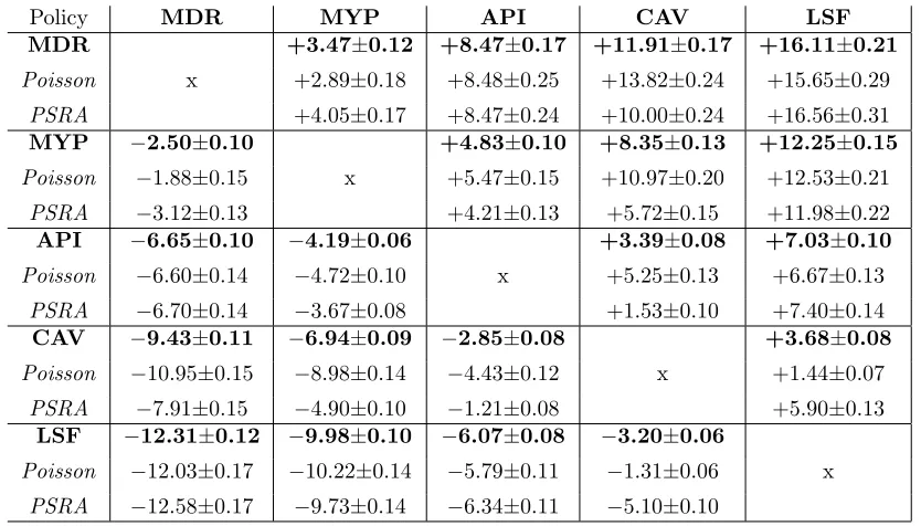
in the table has 3 rows. The first row shows (in bold font) a 95% confidence interval for the percentage increase (or decrease) in the mean total cost when using heuristic ias opposed to heuristic j, taking into account the results from all scenarios. The second row shows an analogous confidence interval for the 50% of scenarios in which customers arrive via nonhomogeneous Poisson processes, and the third row shows the results for the remaining 50% of scenarios in which customers arrive via pre-scheduled random arrival (PSRA) distributions. For clarity, ‘−’ denotes a reduced cost, i.e. an improvement.
Policy MDR MYP API CAV LSF
MDR +3.47±0.12 +8.47±0.17 +11.91±0.17 +16.11±0.21
Poisson x +2.89±0.18 +8.48±0.25 +13.82±0.24 +15.65±0.29
PSRA +4.05±0.17 +8.47±0.24 +10.00±0.24 +16.56±0.31
MYP −2.50±0.10 +4.83±0.10 +8.35±0.13 +12.25±0.15
Poisson −1.88±0.15 x +5.47±0.15 +10.97±0.20 +12.53±0.21
PSRA −3.12±0.13 +4.21±0.13 +5.72±0.15 +11.98±0.22
API −6.65±0.10 −4.19±0.06 +3.39±0.08 +7.03±0.10
Poisson −6.60±0.14 −4.72±0.10 x +5.25±0.13 +6.67±0.13
PSRA −6.70±0.14 −3.67±0.08 +1.53±0.10 +7.40±0.14
CAV −9.43±0.11 −6.94±0.09 −2.85±0.08 +3.68±0.08
Poisson −10.95±0.15 −8.98±0.14 −4.43±0.12 x +1.44±0.07
PSRA −7.91±0.15 −4.90±0.10 −1.21±0.08 +5.90±0.13
LSF −12.31±0.12 −9.98±0.10 −6.07±0.08 −3.20±0.06
Poisson −12.03±0.17 −10.22±0.14 −5.79±0.11 −1.31±0.06 x
[image:26.612.98.515.158.396.2]PSRA −12.58±0.17 −9.73±0.14 −6.34±0.11 −5.10±0.10
Table 1: Pairwise comparisons of the 5 heuristic policies across all 28,800 scenarios
The results indicate that the LSF heuristic performs best, and is able to improve upon the myopic policy by about 10% on average. The CAV heuristic is the second strongest, but (unlike the LSF) appears to become significantly weaker if pre-scheduled arrivals are considered rather than Poisson arrivals. In the PSRA case, the LSF and CAV heuristics both have to estimate a greater number of coefficients in their quadratic approximating functions, and the LSF heuristic seems able to adapt better to this than the more naive CAV heuristic. The API heuristic consistently performs better than the myopic policy, but is usually not able to match the more sophisticated CAV and LSF heuristics. The naive MDR heuristic is not able to perform as well as any of the SAB heuristics. Overall, as expected, the performances of the 4 heuristics are ranked in an order which corresponds with their computational requirements.
We now present further analyses of our numerical results, focusing only on the relative strengths of the 4 SAB heuristics (the naive MDR heuristic will be discussed again later in this section, when different levels of server ‘busyness’ are considered). We can gain greater insight into the relative strengths of the SAB heuristics by breaking down the results according to the values of individual system parameters. Figure 2 shows comparisons between the API, CAV and LSF policies for various different values of β (recall that
β controls the weight of the ‘switching costs’ for changing service rates). The policies are compared with respect to the improvements they achieve against the myopic policy.