Design of an Adaptive Filtering Algorithm for Noise Cancellation

(1)

Page 597

DESIGN OF AN ADAPTIVE FILTERING ALGORITHM FOR NOISE

CANCELLATION

Roshny Jose George

1

_{Guest Assistant Professor, ECE Department, College of Engineering Poonjar, Kerala, India}

---*---Abstract -**

The aim of this paper is to implement a

non-pipelined Least Mean Square (LMS) and a pipelined delayed-LMS (DLMS) adaptive digital Finite Impulse Response (FIR) filters on Field Programmable Gate Array (FPGA) chips for typical noise cancellation applications and compare the behavior of non-pipelined and non-pipelined adaptive algorithms in terms of FPGA resource, speed and area. The direct FIR architecture is considered for non-pipelined filter designing and the transposed FIR architecture is considered for pipelined filter designing. The VHDL hardware description language is used for algorithm modeling and synthesized using XILINX ISE 9.2i on a SPARTAN 3E chip. The obtained results demonstrate that the DLMS algorithm which has pipeline architecture is faster than LMS algorithm while it uses more chip area due to extra registers. The LMS algorithm for adaptive filtering was coded in MATLAB using direct form FIR filter and Signal to Noise Ratio (SNR) of noisy signal and the filtered signals were calculated. Also Mean Square Error (MSE) for different sound signals was determined.

Key Words:

Adaptive Digital Filters, LMS algorithm,

SNR, MSE

1. INTRODUCTION

The usual method of estimating a signal corrupted by additive noise is to pass it through a filter that tends to suppress the noise while leaving the signal relatively unchanged [1]. Filters used for the above purpose can be fixed or adaptive. The design of fixed filters is based on prior knowledge of both the signal and the noise [5]. Adaptive filters, on the other hand, have the ability to adjust their own parameters automatically, and their design requires little or no a priori knowledge of signal or noise characteristics. Here we have to use an adaptive filter for noise cancellation. Noise cancellation is a variation of optimal filtering that involves producing an approximate of the noise by filtering the reference input and then subtracting this noise estimate from theprimary input containing both signal and noise. Adaptive noise cancellation is often used to extract the desired signal

from the given noisy signal. The adaptive filtering operation achieved the best results when system output is noise free. This is achieved by minimizing the mean square value of the error signal. The widely used LMS algorithm is used for the adaptation of the filter coefficients [3]. Since, there is no dedicated IC for adaptive filter; the filter is designed using VHDL code and MATLAB code. An adaptive filtering algorithm is designed in MATLAB using LMS algorithm and SNR of noisy signal and the filtered signals were calculated. In this paper a five tap non-pipelined and non-pipelined adaptive filters were designed. The non-pipelined adaptive filter design uses LMS algorithm and the pipelined adaptive filter design uses the delayed LMS algorithm.

2. ADAPTIVE NOISE CANCELLATION

Noise cancellation technology is a growing field that aims to cancel or at least minimize unwanted signal and so to remedy the excess noise that one may experience. There are already several solutions available. Adaptive noise cancellation [6] is widely used to improve the Signal to Noise Ratio (SNR) of a signal by removing noise from the received signal. In an adaptive noise canceller two input signals are applied simultaneously to the adaptive filter. The signal d =s+n0 is the contaminated signal containing both the desired signal s and the noise n0, assumed uncorrelated with each other. The signal, n1, is a measure of the contaminating signal which correlates in some way with n0. This is the reference input to the canceller. The signal n1 is processed by the digital filter to produce an estimate y, of n0. An estimate of the desired signal, e is then obtained by subtracting the digital filter output, y, from the contaminated signal s+n0 and produce the system output z=s+n0-y [2]. In the adaptive noise cancellation system shown in Figure 1 the desired signal s, is the audio signal and the noise is the signal generated from the Gaussian noise generator.

2.1 Adaptive algorithms

(2)

Page 598

modified version of LMS that is suited for pipelined processing [8].

2.1.1 The LMS algorithm

The easy implementation of the Least Mean Square (LMS) algorithm forms it the best choice for many real-time systems [6]. The algorithm is described by the following equations:

   1

0

i *

) M w_i ( n) x ( n-i)

y( n (1)

(n) - y(n)

e (n) = d (2)

)x( n) ( n) + µe( n i

= w ) ( n+ i

w 1 (3)

In these equations, the tap inputs x (n), x (n-1),.., x (n-M+1) are the elements of the reference signal x (n), where M-1 is the number of delay elements and d (n) denotes the primary input signal, e (n) denotes the error signal and constitutes the overall system output. The term wi (n) denotes the tap weight at the nth iteration. And the scaling factor μ is the step-size parameter. The LMS algorithm is convergent in the mean square if and only if μ satisfies the condition: 0 < μ < 2 / tap-input power.

2.1.2 Delayed LMS algorithm

In some practical applications, the LMS adaptation scheme imposes a critical limit on its implementation. The DLMS is a modified version of LMS that is suited for pipelined processing [8], which provide a high throughput. Compared to the normal LMS algorithm, in DLMS the update coefficient is based on the error D samples before. The algorithm is described by the following equations:

   1

0 M

i * xn-i

n-i i w

y( n) (1)

e(n) = d(n-D) - y(n) (2)

w_i( n+1)=w_i( n)+µe( n-D)x( n-D) (3)

In these equations, d (n-D) denotes the delayed primary input signal, e (n-D) denotes the delayed error signal which constitutes the overall system output and wi(n) denotes the tap weight at the nth iteration.

3. NON PIPELINED LMS ADAPTIVE FILTER

A non-pipelined adaptive filter was designed with a direct‐form FIR filter coded in VHDL using LMS algorithm. Based on the input given, when the train is equal to 1 then this filter will function as an LMS Adaptive Filter or else simple FIR filter. A non-pipelined adaptive filter [10] is divided into four main blocks, i.e. state control, filter output computation, weight update logic and error adjustment module. The Finite state machine (FSM) is

used to design the state control module. The FSM controls the functionality of the adaptive filter [11]. Total six states s0, s1, s2, s3, s4, s5 are specified [11]. Here state s0 is the reset state. Two different commonly used approaches provide the basis of designing FIR filters called direct and transposed architectures. In direct FIR filter the critical path increases linearly as a function of the number of taps. So the maximum clock frequency for long filters is limited.

4. PIPELINED DLMS ADAPTIVE FILTER

Pipelining is the ability to overlap the execution of different instructions at the same time. We can create a pipeline by dividing a complex operation into simpler operations. A pipelined adaptive filter is designed using DLMS algorithm with transposed form FIR filter [12]. It has D units of delay in its error feedback path. Pipelining of the DLMS [9] is obtained by moving these delays and placing them at every tap of the filter, that introduce delays in the coefficients updates. Registers can be added onto the system's reference signal, to align the error signal calculation. Furthermore, weight updates can also be aligned by using delayed filter inputs.

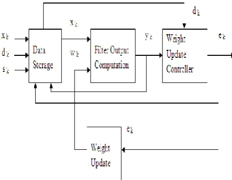
[image:2.595.314.545.459.638.2]

4.1 Block diagram of pipelined adaptive filter

A pipelined adaptive filter block diagram is shown in figure 1 [8]. The filter is divided into four main blocks i.e. data storage, filter output computation, weight update logic and weight update controller.

Fig -1: Block Diagram of pipelined adaptive filter

4.1.1 Data storage Module

(3)

[image:3.595.36.267.77.260.2]

Page 599

Fig -2: Data storage module

4.1.2 Center Tap

A single tap is shown in figure 3. Itconsists of filter output computation and weight update logic modules. This single tap is used in five times for designing a pipelined adaptive filter. The tap processing is pipelined. It means a set of operations connected in series so that the output of one operation is the input of the next one.

Fig -3: Single Tap

(a) Filter Output Computation

The delayed LMS architecture is designed using transposed form FIR filter [13]. The FIR filter design is based on the transposed form in order to keep the maximum data path length short. One advantage of

[image:3.595.310.524.174.355.2]

transposed form over direct form is that transposed FIR filter is self-pipelined. But the area occupied is more than direct form. Pipelining of the adaptive filter is made difficult using LMS algorithm due to the coefficient feedback loop.

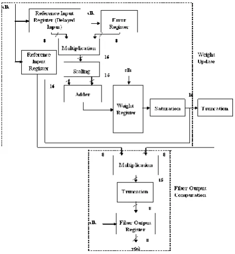
Fig -4: Transposed DLMS Architecture

An architectural implementation of the transposed DLMS is shown in Figure 4, where the algorithm is split into the weight update block and filter block. The filter block of the transposed form is identical to the transposed FIR with fixed coefficient [13].

(b) Weight update logic

A tap consists of weight update module. Here weight update occurred by multiplying the delayed input with error from the error register and the result is multiplied with step size parameter [1]. LMS-like algorithms have a step size that determines the amount of correction applied as the filter adapts from one iteration to the next [1]-[11]. A step size that is too small increases the time for the filter to converge on a set of coefficients or that is too large may cause the adaptive filter to diverge. In that case, the resulting filter might not be stable. So choose smaller step size of 0.0625 for better convergence. Arithmetic Shift Right (ASR) operation is used to simplify and boost the run-time frequency of the design. The output checked for its limit in saturation stage. In this stage the data not to exceed the limit of the coefficient. The saturated data is truncated to 8-bit in next stage. Truncation operation takes places in the weight update component.

(c) Filter Core

[image:3.595.37.269.395.646.2]

(4)

Page 600

[image:4.595.34.274.161.344.2]

The filter output of a tap is the input to the next tap. After tap 5, the output of the filter is obtained and that is used for error calculation.

Fig -5: Filter Core

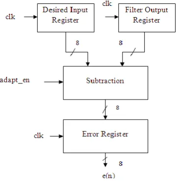
4.1.3 Weight Update Controller

Weight update controller shown in figure 6 can be also termed as an error counting block. The adaptive filter’s output is subtracted from desired signal and produces an error signal. The error signal is stored in an error register and this error signal is fed back to all taps and computes a new coefficient for updating.

Fig -6: Weight Update Controller

5. LMS ALGORITHM IN MATLAB

The LMS algorithm for adaptive filtering was coded in MATLAB using direct form FIR filter and SNR of noisy signal and the filtered signals were calculated [4]. Also MSE for different sound signals were determined [7]. To perform the system improvement signal to noise ratio is

determined and which shows the system effectiveness. The figure of merit used to measure the performance of the adaptive algorithms is the Mean square error or MSE. It is given as





 N

n e n

N MSE

1 ( ) 2 /

1 (1)

In this equation e (n) represents the difference between the original signal and the filtered signal. N is order of the filter.

6. RESULTS

The non- pipelined and pipelined adaptive filters were designed using XILINX ISE software. The hardware implementation of the pipelined adaptive filter is performed in Spartan 3E FPGA kit.

6.1 Simulation results

[image:4.595.308.553.452.582.2]

Human speech signals, acquired through microphones, were used as input signals for the design. The output of the filter is the noise free signal. That is almost equivalent to the original audio signal. To perform the system improvement signal to noise ratio is also determined and which shows the system effectiveness. Figure 7 shows the output of the adaptive filter designed using LMS algorithm in MATLAB. Here the command window shows the SNR of the signals. It shows that SNR of filtered signal is improved.

Fig -7: Output of Adaptive filter in MATLAB

[image:4.595.40.222.475.661.2]

(5)

[image:5.595.37.270.100.188.2]

Page 601

Fig -8: Non- pipelined adaptive Noise Canceller output

Fig -9: Pipelined Adaptive Noise Canceller output

6.2 Implementation results

[image:5.595.37.270.229.325.2]

The aim of this project is to implement the adaptive digital Least Mean Square (LMS) and delayed-LMS (DLMS) Finite Impulse Response (FIR) filters on Field Programmable Gate Array (FPGA) chips for typical noise cancellation applications and compare the behavior of LMS and DLMS adaptive algorithms in terms of chip area utilization and speed. The non- pipelined adaptive filter is designed using XILINX ISE software. The VHDL programs are synthesized separately for each block and the synthesis results observed are shown in below figures.

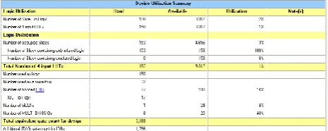
[image:5.595.308.552.426.531.2]

Fig -10: Device utilization summary of non- pipelined adaptive filter

Fig -11: Device utilization summary of pipelined adaptive filter

6.3 Comparison results

The implementation of adaptive digital LMS and DLMS FIR filters on FPGA chips and comparing the behavior of algorithms in terms of chip area utilization and the speed of the filter was proposed. Figure 10 and Figure 11 shows the device utilization summary of two algorithms. According to synthesis resource utilization results, the pipelined adaptive filter utilizes more resources on FPGA than the non-pipelined adaptive filter. The total number of utilized registers for implementing LMS and DLMS adaptive FIR filters is compared. The DLMS adaptive FIR filters need more registers than LMS adaptive FIR filters for providing the delay. Due to extra registers it takes more chip area. In figure 9 the first error output of a non- pipelined adaptive filter is obtained at 1000 ns and the next output is obtained at 2200 ns. Whereas, in figure 10 the first error output of a pipelined adaptive filter is obtained at 380 ns and after that we can get continuous stream of output. The critical path of LMS FIR filters are longer than the DLMS FIR filters. This means that the pipelined DLMS FIR filter is faster than the non-pipelined LMS FIR filter which comes from the pipeline architecture. Table 1 shows the comparison results. It shows that the the pipelined adaptive filter is faster than non pipelined adaptive filter with the usage of large FPGA resources.

Table -1: Comparison results

7. CONCLUSIONS

[image:5.595.36.269.503.596.2] [image:5.595.35.264.635.739.2]

(6)

Page 602

REFERENCES

[1] Mrs. A. B. Diggikar, Mrs. S. S. Ardhapurkar, “Design and Implementation of Adaptive filtering algorithm for Noise Cancellation in speech signal on FPGA” International Conference on Computing, Electronics and Electrical Technologies, 776-771, 2012.

[2] Bernard Widrow, John R. Glover, “Adaptive Noise Cancelling: Principles and Applications”, Proceedings of the IEEE, Vol. 63, No. 12, 1692-1716, 1975.

[3] Simon Haykin. "Adaptive Filters Theory" Pearson Education, 2008.

[4] V.JaganNaveen, T.prabakar, J.Venkata Suman, P.Devi Pradeep, “Noise Suppression in Speech Signals Using Adaptive Algorithms”, International Journal of Signal Processing, Image Processing and Pattern Recognition, Vol. 3, No. 3, 87-96, 2010.

[5] Marvin R, Sambur, “Adaptive Noise Canceling for Speech Signals” , IEEE Transactions on acoustics, speech, and signal processing, vol. assp-26, no. 5, 419-423, 1978.

[6] Mamta M. Mahajan, S. S. Godbole, “Design of Least Mean Square Algorithm for Adaptive Noise Canceller”, International Journal of Advanced Engineering Sciences and Technologies, Vol No. 5, Issue No. 2, 172 – 176, 2011.

[7] Radhika Chinaboina, D.S.Ramkiran, Habibulla Khan, M.Usha, B.T.P.Madhav, “Adaptive Algorithms for Acoustic Echo Cancellation in Speech Processing”, International Journal of Engineering Science and Technology, Vol.3,38-42,2011.

[8] Tadaaki, Kiyoshi, Hitoshi, “An effective architecture of the pipelined LMS adaptive filters”, IEICE Trans.fundamentals, Vol No.8,1428-1434,1999.

[9] Scott C. Douglas, Quanhong Zhu, and Kent F. Smith, “A Pipelined LMS Adaptive FIR Filter Architecture without Adaptation Delay”, IEEE Transactions on signal processing, vol. 46, NO. 3, 775-779, 1998.

[10] S. S. Godbole, P. M. Palsodkar, V. P. Raut, “FPGA Implementation of Adaptive LMS Filter”, Proceedings of SPIT-IEEE Colloquium and International Conference, Vol. 2,226-229,2011. [11] A. B. Diggikar,S.S.Ardhapurkar “Implementing

FSM to control Adaptive Filter for Noise Cancelling in Speech signal”, Proc. of the International Conference on Advanced Computing and Communication Technologies, 452-457,2011. [12] Hesam Ariyadoost, Yousef S. Kavian, Karim Ansari

As “Performance Evaluation of LMS and DLMS Digital Adaptive FIR Filters by Realization on FPGA”, International Journal of Science & Emerging Technologies, Vol-1 No. 1, 7-10, September, 2011.

Design of an Adaptive Filtering Algorithm for Noise Cancellation

Page 597