BIROn - Birkbeck Institutional Research Online
Yakovets, N. and Wang, L. and Fletcher, G. and Taverner, C. and
Poulovassilis, Alexandra (2018) Histogram Domain Ordering for Path
Selectivity Estimation. Proceedings of the 21st International Conference on
Extending Database Technology (EDBT), Vienna, March 26-29, 2018. , pp.
493-496. ISSN 2367-2005.
Downloaded from:
Usage Guidelines:
Please refer to usage guidelines at
or alternatively
Histogram Domain Ordering for Path Selectivity Estimation
Nikolay Yakovets, Li Wang,
George Fletcher
TU Eindhoven, Netherlands
{hush@, l.wang.3@student., g.h.l.
fletcher@}tue.nl
Craig Taverner
Neo4j, Sweden
Alexandra Poulovassilis
Birkbeck, University of London, UK
ABSTRACT
We aim to improve the accuracy of path selectivity estimation
in graph databases by intelligently ordering the domain of a
his-togram used for estimation. This problem has not, to our
know-ledge, received adequate attention in the research community.
We present a novel framework for the systematic study of path
ordering strategies in histogram construction and use. In this
framework, we introduce new ordering strategies which we
ex-perimentally demonstrate lead to significant improvement of the
accuracy of path selectivity estimation over current strategies.
These positive results highlight the fundamental role that domain
ordering plays in the design of effective histograms for efficient
and scalable graph query processing.
1
INTRODUCTION
Analytics on graph-structured data is increasingly important in a
variety of domains, e.g., role discovery in social networks, impact
analysis in citation networks, functional analysis of biological
networks, and querying knowledge graphs. Querying in graph
query languages such as openCypher and PGQL is at the heart of
these analytics tasks [1, 3, 11]. However, current graph database
systems have difficulty in scaling query processing as the size
and complexity of graph data collections continue to grow [4, 9].
Towards addressing this challenge, a crucial step in scalability
of graph databases is the generation of effective query execution
plans. Query optimizers rely on accurate data statistics for
cardin-ality estimation during plan generation. Histograms are among
the most widely used data structure for maintaining statistics
for cardinality estimation, in particular for relational database
systems [5]. However, there has been relatively little work on
histograms for graph queries, even for the most basic graph query
building block, namely, path queries [6–8, 10].
Our contributions.In this paper, we give an overview of find-ings in our ongoing investigations into histograms for path
se-lectivity estimation [12]. We focus in particular on ordering
strategies for path queries, i.e., how to order the domain over
which histograms are built, with the goal of minimizing the
vari-ance within histogram buckets (and thereby improving
estima-tion accuracy). We present a novel framework for systematically
introducing ordering strategies, showing experimentally that
the choice of domain ordering is a fundamental aspect of
effect-ive histograms. We introduce new ordering strategies which we
demonstrate lead to significant improvement on the accuracy of
obtained estimates, over current ordering approaches.
State of the art.The study and efficacy of histogram-based cardinality estimation are well-established [5], e.g., for path and
twig query optimization in XML databases [2, 13]. Several studies
have also considered path selectivity estimation on graph data
© 2018 Copyright held by the owner/author(s). Published in Proceedings of the 21st International Conference on Extending Database Technology (EDBT), March 26-29, 2018, ISBN 978-3-89318-078-3 on OpenProceedings.org.
Distribution of this paper is permitted under the terms of the Creative Commons license CC-by-nc-nd 4.0.
4000
0
label paths 1, 2, 3, 4, 5, 6, 1/1, 1/2, ...
8000
number of pa
ths
1234561/11/21/31/41/51/62/12/22/32/42/52/63/13/23/33/43/53/64/14/24/34/44/54/65/15/25/35/45/55/66/16/26/36/46/56/6
index 1, 2, 3, 4, 5, 6, 7, 8, ...
ranking/ordering 258
[image:2.595.312.538.182.334.2]6/6/6
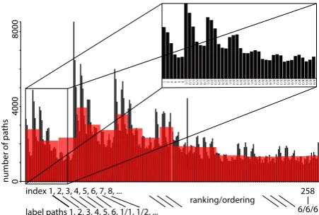
Figure 1: Visualization of a data distribution (black) and an equi-width histogram (red) of Moreno Healthdataset withk=3.
with cycles (i.e., beyond trees and DAGs) [6–8, 10]. These works,
however, have not investigated histograms or the impact of path
ordering on estimation quality. To the best of our knowledge,
we present here the first systematic study of this basic aspect of
histogram construction and use in graph data management.
2
HISTOGRAMS ON LABEL-PATHS
We investigate selectivity estimation of path queries on graphs.
AgraphGis composed of a finite set of verticesV, a set of edge labelsL, and a set of directed labeled edgesE ⊆ V ×L×V. Ak-label pathis a sequenceℓ =l1/. . ./lk, whereli ∈ L, for all 1 ≤ i ≤ k. We sayk = |ℓ|is thelengthofℓ. Viewingℓ as apath query, the evaluation ofℓonGreturns the setℓ(G) consisting of all pairs of vertices(vs,vt)inG such that there exist verticesv0,v1, ...,vk∈Vwherevs =v0,vt =vk, and for 0<i≤k,(vi−1,li,vi) ∈E. The total number of such pairs, i.e., the cardinality ofℓ(G), is called theselectivityofℓonG, which we denote byf(ℓ).
LetLkbe the set of all label paths overLwith length up tok.1 AnorderingofLkis a bijection fromLkto integer set[0,|Lk|). Once we establish an ordering on a label path set, a label path can
be represented by its positional index in the ordering. For each
label pathℓ, letindex(ℓ)denote the index ofℓin the ordering. Ahistogramis a mechanism used to provide the approximation of frequency for a given value (point query) or value range (range
query) without storing or accessing the complete original data
distribution. More precisely, given an attributeX, a histogram on
this attribute is constructed by partitioning the data distribution
of Xintoβ ≥ 1 mutually disjoint subsets calledbuckets and storing the statistics information and bucket boundaries for each
bucket. In this work, attributeX, also called thedomainof the
1
histogram, is an ordered label path sequence produced by an
ordering ofLk. Then, given label pathℓand its indexindex(ℓ), such alabel-path histogramis used to compute an estimatee(ℓ) of the selectivityf(ℓ). An example of a label-path histogram is shown in Figure 1.
3
ORDERING FRAMEWORK
The purpose of histogram domain reordering is to ensure that
label paths with similar cardinality are located close to each other,
such that they can be allocated in the same bucket. This leads to
lower variance, lower error rates, and overall better quality.
An intuitive and ideal way is to arrange the data distribution
such that whenindex(ℓ)increases,f(ℓ)monotonically increases or decreases. The most straightforward, yet not feasible, approach
is to sort the label paths by their selectivity and assign theindex of each label path as its position in this sequence. This idea is not
practical, however, as it requires extra memory to store|L |index values. The exact amount of memory can also be used to store
the cardinality for each label path, such that instead of returning
an estimation of selectivity, we can obtain the precise selectivity.
We call such ordering anideal ordering. Despite an ideal ordering being prohibitive, we can still construct an approximately
mono-tonic sequence based on the awareness of precise cardinalities of
a subset ofL.
For example, by looking at Figure 1, one can observe that the
label1has the highest cardinality among all length-1 label paths while label5has the lowest. Similar trend repeats in the other 6-member groups with the same prefix {1/1, 1/2, . . . , 1/6}, {2/1,
2/2, ..., 2/6}, and so on. Hence, we can assume that the label path
that is composed of label paths with high cardinalities should
also have high cardinality.
3.1
Concepts
We define abase label setas aB ⊆ Lsuch that every label path inLcan be decomposed into pieces which are all inB.2Then, a
splitting ruledefines how to decompose a label path. For example,
L6
onMoreno Healthdataset is {1, 2, 3, 4, 5, 6, 1/1, . . . , 6/6/6/6/6/6},
if we chooseB to beL2, with agreedy splittingrule which at each split step always cuts a piece inBas long as possible. For example, label path “4/4/3/3/6” is decomposed into “4/4”, “3/3”
and “6”.
An ordering method can be described by the following three
components. First, we need a base label setB. Second, we define
(un)ranking functionover the base label set that gives a rank for each base label and vice-versa. It is a bijection which maps
between edge label setBand integer set[1,|B|]. Finally, we con-struct anordering rulewhich is combined with a ranking rule to eventually determine the index of a label path (sequence of base
labels) inLk. It is a bijection that maps between label path setL and integer set[0,|Lk|). A complete ordering method, therefore, is seen as the combination of a ranking rule and an ordering
rule on a given dataset. We refer to an ordering method that is
composed of ranking ruleAand ordering ruleBasB-Aordering. We define two ranking rules in our study.Alphabetical ranking assigns ranks based on the alphabetical order of base labels.
Car-dinality rankingis ranking based on the cardinality of base labels, which places a base label with lower cardinality in front of the
label with higher cardinality, i.e.,l1<cardl2 ⇐⇒ f(l1)<f(l2)
2
Naturally,L⊆B, otherwise there might exist label paths which cannot be decomposed into label paths inB.
In this work, we focus on the approach that takes the edge
label set as the base label set, i.e.,B=L. We define two bijections:
alphandcard. Letalph(l)andcard(l)denote the index of edge labell, which will be referred to as therankofl, in the setLtotally ordered by alphabetical order and cardinality, respectively.
3.2
Numerical and Lexicographical Orderings
In numerical ordering, each rank is an integer, and a composition
of ranks produces a number in|B|-based numeral system. For example, to compare two label paths ℓ1 = l1
1/l 1 2/. . ./l
1
m and ℓ2=l
2 1/l
2 2/. . ./l
2
n, if one is shorter than the other then it has a lower ranking (rule (1) below), otherwise the two paths’ labels
are compared pairwise until a pair of different values is found at
positioni(rule (2) below):
ℓ1< ℓ2 ⇐⇒
(
|ℓ1|<|ℓ2| |ℓ1|,|ℓ2|(1)
∧i−1
j=1(l 1
j =l2j) ∧ (li1<li2) |ℓ1|=|ℓ2|(2) Lexicographical ordering is the same as the ordering rule used
in dictionaries; it is similar to numerical ordering with the
fol-lowing difference. Instead of comparing lengths of two label
paths first, we appendk− |ℓ|blanksymbols (i.e., special symbols for which∀l ∈L,rank(blank) >rank(l)) to everyℓto form a length-ksequence. We can then apply Formula 2 to compare the resulting label paths. The time complexity of both ranking and
unranking functions for numerical and lexicographical orderings
isO(k).
3.3
Sum-based Ordering
Given label pathℓ, the idea ofsum-basedordering is to use the sum of ranks of all base labels inℓto approximate the cardinality
ofℓ. While being conceptually simple, the implementation of this
ordering method is not trivial. First, given a path labelℓof length
k,ℓis split into base labels and an integer rank is computed for each of the base labels to obtain ak-length integerpermutation. Then, the integer permutation ofℓis mapped toindex(ℓ)by performing athree-stage partitioningof a histogram domain as follows.
The first stage partitions the histogram domain according to
the length of the integer permutations, with shorter lengths being
assigned partitions with lower indexes in the domain. Then, the
size of each of the stage-one partitions can be computed by the
following formula (wherenis the length of the permutation):
sumn=|L|n
The second stage performs further division of stage-one
par-titions by grouping allm-length permutations by theirsummed
ranks. Those permutations with lower summed rank will have a lower index within a stage-one partition:
srm = m−1
Õ
i=0
rank(li)
To compute the boundaries of each of the stage-two partitions,
we need to determine how many label paths are in the group
with a certainmandsrm. This question is the same as how many ways there are to distributesrmindistinguishable balls overm distinguishable bins of finite capacity|L|with at least one ball in each bin. From combinatorics’inclusion−exclusion principlewe have:
dist(srm,m,L)=Õ
j≥0
(−1)j
m j
srm−j· |L| −1
m−1
The third stage explores combinations inside each of the
stage-two partitions marked by lengthmand summed ranksrm. These combinations are allinteger partitionsofsrminto exactlymparts, where each part is less than|L|. Let integersv,brepresentsrmand
|L|respectively. A general formula for integer partitionip(v,b,m) is as follows:
ip(v,m,b)=
⌊v/b⌋
Ø
i=0
ip(v−i·b,m−1,b−1),b,· · ·,b
| {z }
ibs (4)
Based on Formula 4, we present a partitioning algorithm which
outputs all combinations in the desired cardinality-based order
and has time complexity isO(loд(|L|)k)[12].
Finally, to compute the boundaries of each of the stage-three
partitions, we need to determine how many permutations we
skip when we skip a stage-three partition. This is equivalent
to identifying how many permutations can be generated by a
certain combination in which there might be duplicates. LetC denote the combination,didenote the number of times an integer
ioccurs inC, then the number of permutations is given by the following formula:
nop(C)= |C|!
Î
i∈ {0, ...,|L|−1}
di!
(5)
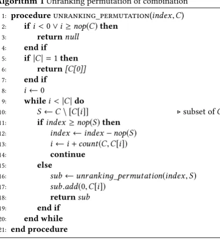
Algorithm 1 finds the combination to which the target
per-mutation belongs and has time complexity ofO(k2).
Algorithm 1Unranking permutation of combination
1: procedureunranking_permutation(index,C) 2: ifi<0∨i≥nop(C)then
3: returnnull 4: end if
5: if|C|=1then
6: return[C[0]] 7: end if
8: i←0
9: whilei<|C|do
10: S←C\ [C[i]] ▷subset ofC
11: ifindex ≥nop(S)then 12: index←index−nop(S) 13: i←i+count(C,C[i])
14: continue
15: else
16: sub←unrankinд_permutation(index,S)
17: sub.add(0,C[i])
18: returnsub
19: end if
20: end while 21: end procedure
Algorithm 2 illustrates the complete version of unranking
permutation in sum-based order and has time complexity of
O(loд(|L|)k).
3.4
Ordering Example
We illustrate the proposed ordering methods with examples on an
artificial dataset which has 3 unique edge labels and its label paths
set withkup to 2. Consider the cardinalities 20,100, and 80 for edge labels “1”, “2”, and “3”, respectively. Then, for the summed
ranks shown in Table 1, label paths arranged in the corresponding
Algorithm 2Unranking in sum-based order
1: procedureunranking_in_sumbased(index,L,k) ▷index, edge label set, k
2: ifindex<0∨index >|Lk|then 3: returnnull
4: end if
5: forlen∈1, ...,kdo 6: ifindex≥ |L|lenthen 7: index←index− |L|len
8: continue
9: end if
10: forsum∈len, ...,len∗ |L|do 11: ifindex ≥dist(sum,len,|L|)then 12: index ←index−dist(sum,len,|L|)
13: continue
14: end if
15: P←ip(sum,len,|L|)
16: forp∈Pdo
17: ifindex ≥nop(p)then 18: index←index−nop(p)
19: continue
20: end if
21: p′← {i−1|i∈p}
22: sort(p′)
23: returnunrankinд_permutation(index,p′)
24: end for
25: end for
26: end for
27: end procedure
Label Path 1 2 3 1,1 1,2 1,3 2,1 2,2 2,3 3,1 3,2 3,3
[image:4.595.308.544.80.573.2]Summed Ranks 1 3 2 2 4 3 4 6 5 3 5 4
Table 1: Summed ranks
O
Index
0 1 2 3 4 5 6 7 8 9 10 11
num-alph 1 2 3 1,1 1,2 1,3 2,1 2,2 2,3 3,1 3,2 3,3
num-card 1 3 2 1,1 1,3 1,2 3,1 3,3 3,2 2,1 2,3 2,2
lex-alph 1 1,1 1,2 1,3 2 2,1 2,2 2,3 3 3,1 3,2 3,3
lex-card 1 1,1 1,3 1,2 3 3,1 3,3 3,2 2 2,1 2,3 2,2
[image:4.595.58.283.395.640.2]sum-based 1 3 2 1,1 1,3 3,1 3,3 1,2 2,1 3,2 2,3 2,2
Table 2: Ordered label paths according to different order-ing methodsO
orderings are shown in Table 2. Respectively, numerical ordering
associated with alphabetical ranking, numerical ordering with
cardinality ranking, lexicographical ordering with alphabetical
ranking, lexicographical ordering with cardinality ranking,
sum-based ordering with cardinality ranking are referred to as
num-alph,num-card,lex-alph,lex-cardandsum-based.
4
EXPERIMENTAL STUDY
We implemented ak-path histogram construction and path se-lectivity estimation in Java. All experiments are conducted on an
Ubuntu 16.04 machine equipped with an Intel i5 CP U with 4GB
of RAM. We use the datasets shown in Table 3. The goal of our
experiments is two-fold. First, we verify the impact of different
domain ordering techniques on the estimation time. Second, we
showcase the gains in estimation accuracy which can be obtained
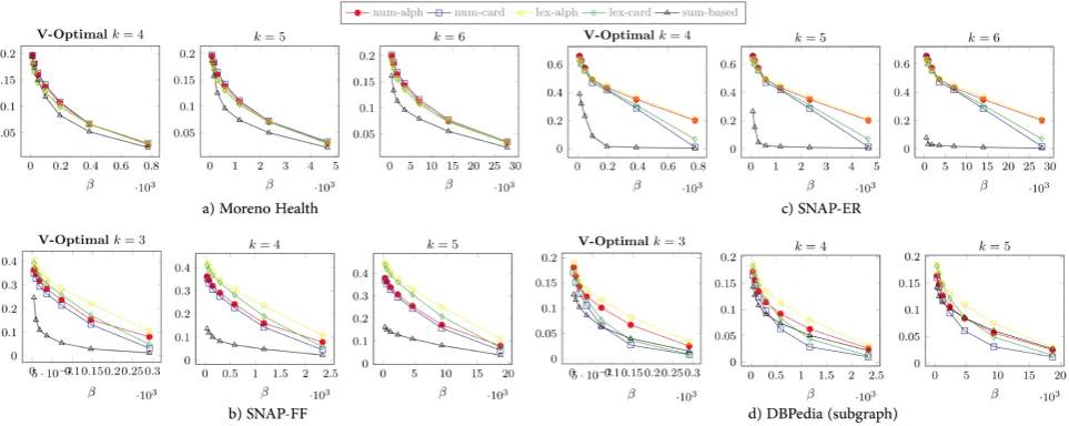
Figure 2: Mean error rate of estimation for different domain ordering techniques on V-Optimalk-path histogram
Dataset #Edge Labels #Vertices #Edges Real world data
Moreno health3 6 2539 12969 yes
DBpedia (subgraph)4 8 37374 209068 yes SNAP-ER5 6 12333 147996 no
SNAP-FF 8 50000 132673 no
Table 3: Datasets
[image:5.595.53.287.317.483.2]β Average Estimation Running Time (in ms) num-alph num-card lex-alph lex-card sum-based 27993 9.98 8.62 9.65 8.7 11.02 13996 7.69 7.23 7.79 7.3 9.39 6998 7.36 6.8 7.07 6.93 8.55 3499 6.4 6.52 5.97 6.31 7.42 1749 5.71 5.76 5.76 5.21 6.64 874 5.8 5.06 5.78 5.18 6.1 437 5.19 4.58 4.52 4.29 6.13 Table 4: Average estimation execution time in V-optimal histogram with different ordering methods (in ms)
Performance. We study the execution time of estimation asso-ciated with different ordering methods as follows. Fork=6, five V-optimal histograms are built, each of which is associated with
an ordering method:num-alph,num-card,lex-alph,lex-card, and
sum-based. The total number of label paths is 55996. We run 7 experiments by varying the number of buckets (β) in each histo-gram. All experiments are executed 100 times and the average
estimation time is taken. The results (Table 4) demonstrate that
sum-based ordering is approximately 20% slower in estimation
than native ordering methods. This is explained by the higher
complexity of the sum-based (un)ranking function.
Accuracy. We measure the average estimation accuracy by con-structing a V-optimal histogram for each ordering method for
varyingkandβ(Figure 2). We use the followingerr(ℓ)metric to measure the error of an estimation:
err(ℓ)=
(
0 if e(ℓ)=f(ℓ)
e(ℓ)−f(ℓ)
max(e(ℓ),f(ℓ)) else
(6)
3
http://konect.uni- koblenz.de/networks/moreno_health
4
http://wiki.dbpedia.org
5https://snap.stanford.edu/snappy/
We observe that, for the synthetic datasets, sum-based
order-ing provides accuracy which is far superior to other orderorder-ing
methods, especially, for histograms with a low number of
buck-ets. For the real-life datasets, the performance difference is not
as significant, but still observable. This can be explained by the
presence of edge-label cardinality correlations in real-life data.
5
CONCLUDING REMARKS
We have reported on initial findings in our ongoing study of
domain ordering for improving histogram-based path selectivity
estimation. Experimental study has demonstrated the promise of
our framework, which facilitates the further systematic study of
effective histogram design for graph databases. A primary future
research direction is to expand the framework with additional
ordering strategies, e.g., those built over richer base sets such as
L2
, towards capturing correlations between label paths.
REFERENCES
[1] 2017. openCypher. (2017). https://www.opencypher.org/
[2] A. Aboulnaga, A. Alameldeen, and J. Naughton. 2001. Estimating the selectivity of XML path expressions for internet scale applications. InVLDB. 591–600. [3] Renzo Angles et al. 2018. G-CORE: A core for future graph query languages.
InSIGMOD 2018. to appear.
[4] G. Bagan, A. Bonifati, R. Ciucanu, G. Fletcher, A. Lemay, and N. Advokaat. 2017. gMark: Schema-driven generation of graphs and queries.IEEE Trans.
Knowl. Data Eng.29, 4 (2017), 856–869.
[5] G. Cormode et al. 2012. Synopses for massive data: samples, histograms, wavelets, sketches.Found. Trends Data.4, 1-3 (2012), 1–294.
[6] George H. L. Fletcher, Jeroen Peters, and Alexandra Poulovassilis. 2016. Effi-cient regular path query evaluation using path indexes. InEDBT 2016. 636–639. [7] T. Neumann and G. Moerkotte. 2011. Characteristic sets: Accurate cardinality
estimation for RDF queries with multiple joins. InICDE 2011. 984–994. [8] Yun Peng, Byron Choi, and Jianliang Xu. 2011. Selectivity estimation of twig
queries on cyclic graphs. InICDE 2011. 960–971.
[9] Siddhartha Sahu, Amine Mhedhbi, Semih Salihoglu, Jimmy Lin, and M. Tamer Özsu. 2017. The ubiquity of large graphs and surprising challenges of graph processing.PVLDB11 (2017), 420 – 431. Issue 4.
[10] Silke Trißl and Ulf Leser. 2010. Estimating result size and execution times for graph queries. InGraphQ 2010. 11–20.
[11] Oskar van Rest, Sungpack Hong, Jinha Kim, Xuming Meng, and Hassan Chafi. 2016. PGQL: a property graph query language. InGRADES 2016.
[12] Li Wang. 2017.On histograms for path selectivity estimation in graph data. Master’s thesis. Eindhoven University of Technology.