Randomness Efficient Curve Sampling

Randomness-efficient Curve Sampling

Thesis by

Zeyu Guo

In Partial Fulfillment of the Requirements for the

Master Degree in Computer Science

California Institute of Technology Pasadena, California

2014

c

2014

Abstract

Curve samplers are sampling algorithms that proceed by viewing the domain as a vector space over a finite field, and randomly picking a low-degree curve in it as the sample. Curve samplers exhibit a nice property besides the sampling property: the restriction of low-degree polynomials over the domain to the sampled curve is still low-degree. This property is often used in combination with the sampling property and has found many applications, including PCP constructions, local decoding of codes, and algebraic PRG constructions.

The randomness complexity of curve samplers is a crucial parameter for its applications. It is known that (non-explicit) curve samplers usingO(logN + log(1/δ)) random bits exist, where N is the domain size and δ is the confidence error. The question of explicitly con-structing randomness-efficient curve samplers was first raised in [TSU06] where they obtained curve samplers with near-optimal randomness complexity.

Contents

Abstract iii

1 Introduction 1

2 Preliminaries 7

3 Basic results 16

3.1 Extractor vs. sampler connection . . . 16

3.2 Existence of a good curve sampler . . . 17

3.3 Lower bounds . . . 18

4 Explicit constructions 20 4.1 Outer sampler . . . 20

4.1.1 Block source conversion . . . 20

4.1.2 Block source extraction . . . 24

4.2 Inner sampler . . . 26

4.2.1 Error reduction . . . 26

4.2.2 Iterated sampling . . . 29

4.2.3 Recursive inner sampler . . . 31

4.3 Putting it together . . . 34

4.4 An alternative outer sampler . . . 35

Chapter 1

Introduction

Overview

Randomness has numerous uses in computer science, and sampling is one of its most classical applications: Suppose we are interested in the size of a particular subset A lying in a large domain D. Instead of counting the size of A directly by enumeration, one can randomly draw a small sample fromDand calculate the density ofAin the sample. The approximated density is guaranteed to be close to the true density (measured by a parameter, theaccuracy error) with probability 1−δ where δ is very small, known as the confidence error. This sampling technique is extremely useful both in practice and in theory.

One class of sampling algorithms, known as curve samplers, proceed by viewing the domain as a vector space over a finite field, and picking a random low-degree curve in it. Curve samplers exhibit the following nice property besides the sampling property: the restriction of low-degree polynomials over the domain to the sampled curve is still low-degree. This special property, combined with the sampling property, turns out to be useful in many settings, e.g local decoding of Reed-Muller codes and hardness amplification [STV01], PCP constructions [AS98, ALM+_{98, MR08], algebraic constructions of pseudorandom-generators}

[SU05, Uma03], extractor constructions [SU05, TSU06], and some pure complexity results (e.g. [SU06]).

the confidence error. The real difficulty, however, is to find an explicit construction matching this bound.

Previous work

Randomness-efficient samplers (without the requirement that the sample points form a curve) are constructed in [CG89, Gil98, BR94, Zuc97]. In particular, [Zuc97] obtains explicit sam-plers with optimal randomness complexity (up to a 1 +γ factor for arbitrary small γ >0) using the connection between samplers and extractors. See [Gol11] for a survey of samplers. Degree-1 curve samplers are also called line samplers. Explicit randomness-efficient line samplers are constructed in the PCP literature [BSSVW03, MR08], motivated by the goal of constructing almost linear sized PCPs. In [BSSVW03] line samplers are derandomized by picking a random point and a direction sampled from an -biased set, instead of two random points. An alternative way is suggested in [MR08] where directions are picked from a subfield. It is not clear, however, how to apply these techniques to higher degree curves.

In [TSU06] it was shown how to explicitly construct derandomized curve samplers with near-optimal parameters by employing an iterated sampling technique. Formally they ob-tained

• curve samplers picking curves of degree (log logN + log(1/δ))O(log logN) using random-ness O(logN+ log(1/δ) log logN), and

• curve samplers picking curves of degree (log(1/δ))O(1) using randomness O(logN + log(1/δ)(log logN)1+γ) for any constant γ >0

for domain sizeN, field sizeq≥(logN)Θ(1)_{and confidence errorδ=N}−Θ(1)_{. Their work left}

the problem of explicitly constructing low-degree curve samplers (ideally picking curves of degreeO(log_q(1/δ))) with essentially optimalO(logN+log(1/δ)) random bits as a prominent open problem.

Main results

It is known that curve samplers in _Fm_q must have sample complexity Ω

log(/δ)

2

and ran-domness complexity (m−1) logq+ log (1/) + log (1/δ)−O(1) [RTS00]. It is also not hard to show that the degree of the sampled curves has to be Ω log_q(1/δ) (c.f. Theorem 3.3.3). We construct explicit curve samplers with parameters that match or are close to these lower bounds. In particular, we show how to sample degree- mlog_q(1/δ)O(1) curves in _Fm

q using

O(logN+ log(1/δ)) random bits for domain sizeN =|_Fm

Before stating our main theorem, we first present the formal definition of samplers and curve samplers.

Samplers. Given a finite set Mas the domain, the density of a subsetA ⊆ M isµ(A)def=

|A|

|M|. For a collection of elements T = {ti :i ∈I} ∈ M

I _{indexed by set I, the density of A}

inT isµT(A) def

= |A_{|T |}∩T | = Pri∈I[ti ∈A].

Definition 1.0.1 (sampler). A sampler is a function S : N × D → M where |D| is its sample complexity and M is its domain. We say S samples A ⊆ M with accuracy error and confidence error δ if

Pr

x∈N[|µS(x)(A)−µ(A)|> ]≤δ

where S(x) def= {S(x, y) : y ∈ D}. We say S is an (, δ) sampler if it samples all subsets A ⊆ M with accuracy error and confidence error δ. The randomness complexity of S is log(|N |).

Lines, curves, and manifolds. To define curve sampler, we first define curves, lines, and more generally manifolds. Let f : _Fd

q → FDq be a map. We may view f as D individual

functions fi : Fdq → Fq describing its operation on each output coordinate, i.e., f(x) =

(f1(x), . . . , fD(x)) for allx∈Fdq.

Definition 1.0.2 (manifold). A manifold in_FD_q is a functionC :_Fd_q →_FD

q whereC1, . . . , CD

are d-variate polynomials over_Fq. We call d the dimension of C. We say a manifold C has

degreetif each polynomialCi has degreet. An 1-dimensional manifold is also called acurve.

A curve of degree 1 is also called a line.

Now we are ready to define curve samplers, the central objects studied in this thesis.

Definition 1.0.3(curve/line sampler). LetM=_FD_q andD =_Fq. The samplerS :N ×D →

M is a degree-t curve sampler if for all x∈ N, the function S(x,·) : D → M is a curve of degree at most t over _Fq. When t= 1, S is also called a line sampler.

The main result of this thesis is as follows.

Theorem 1.0.1 (main). For any , δ > 0, integer m ≥ 1, and sufficiently large prime power q ≥mlog(1 /δ)Θ(1), there exists an explicit degree-t curve sampler for the domain _Fm q

with t = mlog_q(1/δ)O(1), accuracy error , confidence error δ, sample complexity q, and randomness complexity O(mlogq+ log(1/δ)) = O(logN + log(1/δ)) where N = qm is the domain size. Moreover, the curve sampler itself has degree mlog_q(1/δ)O(1)

Theorem 1.0.1 has better degree bound and randomness complexity compared with the constructions in [TSU06]. The degree bound, being mlog_q(1/δ)O(1)

, is still sub-optimal compared with the lower bound log_q(1/δ). However, we remark that in typical settings it is satisfying to to achieve such a degree bound.

As an example, consider the following setting of parameters: domain size N =qm_{, field}

size q = (logN)Θ(1), confidence error δ = N−Θ(1)_{, and accuracy error = (logN)}−Θ(1)

. Note that this is the typical setting in PCP and other literature [ALM+_{98, AS98, STV01,}

SU05]. In this setting, we have the following corollary in which the randomness complexity is logarithmic and the degree is polylogarithmic.

Corollary 1.0.1. Given domain sizeN =|_Fm

q |, accuracy error = (logN)

−Θ(1)

, confidence error δ=N−Θ(1), and large enough field sizeq= (logN)Θ(1), there exists an explicit degree-t curve sampler for the domain_Fm_q with accuracy error , confidence errorδ, randomness com-plexity O(logN), sample complexityq, andt≤(logN)cfor some constant c >0independent of the field size q.

It remains an open problem to explicitly construct curve samplers that have optimal randomness complexity O(logN + log(1/δ)) (up to a constant factor), and sample curves with optimal degree bound O(log_q(1/δ)). It is also an interesting problem to achieve the optimal randomness complexity up to a 1 +γ factor for any constantγ >0 (rather than just an O(1) factor), as achieved by [Zuc97] for general samplers. The standard techniques in [Zuc97] are not directly applicable as they increase the dimension of samples and only yield O(1)-dimensional manifold samplers.

Techniques

Extractor machinery. It was shown in [Zuc97] that samplers are equivalent to extrac-tors, objects that convert weakly random distributions into almost uniform distributions. Therefore the techniques of constructing extractors are extremely useful in constructing curve samplers. Our construction employs the technique of block source extraction [NZ96, Zuc97, SZ99]. In addition, we also use the techniques appeared in [GUV09], especially their constructions ofcondensers.

Iterated sampling. Iterated sampling is a useful technique for explicitly constructing randomness-efficient samplers [BR94, TSU06]. The idea is first picking a large sample from the domain and then draw a sub-sample from the previous sample. The drawback of iter-ated sampling, however, is that it invests randomness twice while the confidence error does not shrink correspondingly. To remedy this problem, we add another ingredient into our construction, namely the technique of error reduction.

Error reduction via list-recoverable codes. We will use explicit list-recoverable codes (a strengthening of decodable codes [GI01]). More specifically, we will employ the list-recoverability from (folded) Reed-Solomon codes [GR08, GUV09]. List-recoverable codes provide a way of obtaining samplers with very small confidence error from those with mildly small confidence error. We refer to this transformation aserror reduction, which plays a key role in our construction.

Sketch of the construction

Our curve sampler is the composition of two samplers which we call the outer sampler and the inner sampler respectively. The outer sampler picks manifolds of dimension O(logm) from the domainM=_Fm

q . The outer sampler has near-optimal randomness complexity but

the sample complexity is large. To fix this problem, we employ the idea of iterated sampling. Namely we regard the manifold picked by the outer sampler as the new domain M0_{, and}

then construct an inner sampler picking a curve from M0 _{with small sample complexity.}

The outer sampler is obtained by constructing an extractor and then using the extractor-sampler connection [Zuc97]. We follow the approach in [NZ96, Zuc97, SZ99]: Given an arbitrary random source with enough min-entropy, we will first use a block source converter to convert it into ablock source, and then feed it to ablock source extractor. In addition, we need to construct these components carefully so as to maintain the low-degree-ness. The way we construct the block source converter is different from those in [NZ96, Zuc97, SZ99] (as they are not in the form of low-degree polynomial maps), and is based on the Reed-Solomon condenser proposed in [GUV09]: To obtain one block, we simply feed the random source and a fresh new seed into the condenser, and let the output be the block. We show that this indeed gives a block source.

complexity, whereas error reduction reduces the confidence error but increases the sample complexity. Our construction applies the two techniques alternately such that (1) we keep the invariant that the confidence error is always exponentially small in the randomness com-plexity, and (2) the sample complexity is finally brought down to q. We remark that the idea of sandwiching several operations to get the desired parameters without spoiling other ones is reminiscent of Reingold’s proof that SL = L [Rei08] and Dinur’s proof of the PCP theorem [Din07].

Outline

Chapter 2

Preliminaries

Notations and basic definitions

We denote the set of numbers {1,2, . . . , n} by [n]. Given a prime power q, write _Fq for the

finite field of size q. Write US for the uniform distribution over a finite set S, Un,q for the

uniform distribution over _Fn_q, and Un for the uniform distribution over{0,1}n. Logarithms

are taken with base 2 unless the base is explicitly specified.

Random variables and distributions are represented by upper-case letters whereas their specific values are represented by lower-case letters. Write x←X if x is sampled according toX. Write X ⊂S if X is a distribution over a set S. The support of a distributionX ⊂S is supp(X) def= {x ∈ S : Pr[X = x] > 0}. We use the statistical distance ∆(·,·) to measure the closeness of two distributions. The statistical distance between X, Y ⊂S is defined as

∆(X, Y) = max

T⊆S |Pr[X ∈T]−Pr[Y ∈T]|.

Then ∆(·,·) defines a metric. We say X is -close toY if ∆(X, Y)≤.

Fact 1. The statistical distance is half the `1 distance, i.e., for X, Y ⊂S, we have

∆(X, Y) = 1 2

X

x∈S

|Pr[X =x]−Pr[Y =x]|.

For an event A, let I[A] be the indicator variable that evaluates to 1 if A occurs and 0 otherwise. For a distributionX and an eventA that occurs with nonzero probability, define the conditional distribution X|A by Pr[X|A=x] = Pr[(X_Pr[=_Ax_])∧A].

We use forms like {tx : x ∈ I} ∈ SI to denote a collection of elements indexed by I

with each element in the set S. Alternatively, we view {tx : x ∈ I} as the function from

(unordered) multi-set.

Indeterminates are written as upper-case letters. E.g., we use _F[X1, . . . , Xn] to denote

the polynomial ring over the field _F with indeterminates X1, . . . , Xn. We say a polynomial

p(X1, . . . , Xn) has degree t if the sum of the individual degrees Pn_i=1ai is at most t for all

monomial Qn i=1X

ai

i of p.

Facts about curves and manifolds

Fact 2. For any distinct x1, . . . , xt+1 ∈ Fq and any y1, . . . , yt+1 ∈ Fnq, there exists a unique

curve C :_Fq →Fnq of degree t such that C(xi) = yi for all i∈[t+ 1]. Indeed, Ci’s are given

by the Lagrange polynomials:

Ci(X) = t+1

X

j=1

yj,i

Y

k∈[t+1]\{j}

X−xk

xj −xk

where yj,i is the i-th coordinate of yj, i∈[n].

Fact 3. Let f1 : Fdq1 → Fdq0 be a manifold of degree t1 and f2 : Fdq2 → Fdq1 a manifold of

degree t2. Then f1◦f2 :Fqd2 →Fdq0 is a manifold of degree t1t2.

We also need the following lemma, generalizing the one in [TSU06]:

Lemma 2.0.1. A manifold f : _FqD

n

→ _FqD

m

of degree t, when viewed as a function f : _FD_qn → _FD

q

m

, is also of degree t.

Proof. Write f = (f1, . . . , fm). By symmetry we just show f1, when viewed as a function

f1 : FDq

n

→_FD

q, has degree t. Suppose

f1(x1, . . . , xn) =

X

d=(d1,...,dn)

P

di≤t

cd n

Y

i=1

xidi.

Let (e1, . . . , eD) be the standard basis of FDq over Fq. Writing the i-th variable xi ∈FqD as

PD

j=1xi,jej ∈ FqD with xi,j ∈Fq, and each coefficient cd ∈FqD as PD_j=1c_d,je_j with c_d,j ∈_Fq,

we obtain

f1(x1, . . . , xn) =

X

d=(d1,...,dn)

P

di≤t

D

X

j=1

cd,jej

! _n Y i=1 D X j=1

xi,jej

!di

.

After multiplying out, each monomial has degree at most maxdP_idi ≤ t, and their

(e1, . . . , eD) and gathering the coefficients onei, we obtain the i-th coordinate function off1

that has degree at most d for all 1 ≤ i ≤ D. Therefore f1 : FDq

n

→ _FD

q is a manifold of

degree t, and so is f : _FD q

n

→ _FD

q

m .

Tail probability bounds

We say random variables X1, . . . , Xn are independent if for any specific values x1, . . . , xn, it

holds that

Pr " _n

^

i=1

Xi =xi

# =

n

Y

i=1

Pr[Xi =xi].

We say X1, . . . , Xn are pairwise independent if for any specific valuesx1, x2 and any distinct

i1, i2 ∈[n], it holds that

Pr [Xi1 =x1∧Xi2 =x2] = Pr[Xi1 =x1] Pr[Xi2 =x2].

In general, for an integer t >1, we say X1, . . . , Xn are t-wise independentif for any specific

values x1, . . . , xt and any distinct i1, . . . , it∈[n], it holds that

Pr " _t

^

j=1

Xij =xj

# =

t

Y

j=1

Pr[Xij =xj].

We consider the behaviour of a fully random curve C of degree t over _Fq, i.e., write

C = (C1, . . . , Cn), then each Ci is a degree-t univariate polynomial whose t+ 1 coefficients

are chosen uniformly at random from _Fq, and allCi’s are chosen independently. It is known

that the points onC are (t+ 1)-wise independent.

Lemma 2.0.2. Let C : _Fq → Fnq be a random curve of degree t over Fq. Then the random

variables C(x)’s are (t+ 1)-wise independent where x ranges over _Fq.

Proof. First note that each C(x) is uniformly distributed. By Fact 2, for any distinct y1, . . . , yt+1 ∈ Fq and any z1, . . . , zt+1 ∈ Fnq, there is a unique degree-t curve, out of all

q(t+1)n _{curves, that passes z}

i at yi for all i∈[t+ 1]. So we have

Pr "_t+1

^

i=1

C(yi) = zi

#

= 1

q(t+1)n = t+1

Y

i=1

Pr[C(yi) =zi].

By definition, the random variables C(x)’s with xranging over _Fq are (t+ 1)-wise

We need the Chernoff bound of the following form:

Lemma 2.0.3. Suppose X1, . . . , Xn ⊂ [0,1] are independent random variables. Let X =

Pn

i=1Xi and µ=E[X], and let R ≥6µ. Then

Pr[X ≥R]≤2−R. The following bound follows from Chebyshev’s inequality:

Lemma 2.0.4. Suppose X1, . . . , Xn are pairwise independent random variables. Let X =

Pn

i=1Xi and µ=E[X], and let A >0. Then

Pr[|X−µ| ≥A]≤

Pn

i=1Var[Xi]

A2 .

We will also use the following tail bound for t-wise independent random variables:

Lemma 2.0.5 ([BR94]). Let t ≥ 4 be an even integer. Suppose X1, . . . , Xn ⊂ [0,1] are

t-wise independent random variables. Let X =Pn

i=1Xi and µ=E[X], and let A >0. Then

Pr[|X−µ| ≥A] =O

tµ+t2

A2

t/2! .

Basic line/curve samplers

The simplest line samplers are those picking completely random lines, as defined below. We call them as basic line samplers.

Definition 2.0.4(basic line sampler). Form≥1 and prime powerq, letLinem,q :F2qm×Fq →

Fmq be the line sampler that picks a uniformly random line inFmq . Formally,

Linem,q((a, b), y)

def

= (a1y+b1, . . . , amy+bm)

for a= (a1, . . . , am), b= (b1, . . . , bm)∈Fmq and y∈Fq.

Remark 1. Note that although Linem,q(x,·) is a line (i.e., a degree-1 curve) for x∈F2qm, the

function Linem,q itself is a degree-2 manifold.

The basic line samplers are indeed good samplers:

Lemma 2.0.6. For >0, m≥1 and prime power q, Linem,q is an

, 1

2_q

Proof. Let A be an arbitrary subset of _Fm

q . Note that Linem,q picks a line uniformly at

random. By Lemma 2.0.2, the random variablesLinem,q(U2m,q, y) with yranging overFq are

pairwise independent. So the indicator variablesI[Linem,q(U2m,q, y)∈A] with yranging over

Fq are also pairwise independent. Applying Lemma 2.0.4, we get

Pr

x←U2m,q

µLinem,q(x,·)(A)−µ(A)

> = Pr   X

y∈_Fq

I[Linem,q(U2m,q, y)∈A]−E



 X

y∈_Fq

I[Linem,q(U2m,q, y)∈A]

  > q   ≤ P

y∈FqVar

I[Linem,q(U2m,q, y)∈A]

2_q2

≤ 1

2_q.

By definition,Linem,q is an

,12_q

line sampler.

Similarly we consider the simplest low-degree curve samplers that pick completely random curves. We call them basic curve samplers.

Definition 2.0.5 (basic curve sampler). Form ≥1,t ≥4 and prime powerq, letCurvem,t,q :

Ftmq ×Fq →Fmq be the curve sampler that picks a uniformly random curve of degreet−1 in

Fmq . Formally,

Curvem,t,q((c0, . . . , ct−1), y)

def

=

t−1

X

i=0

ci,1yi, . . . ,

t−1

X

i=0

ci,myi

!

for each c0 = (c0,1, . . . , c0,m), . . . , ct−1 = (ct−1,1, . . . , ct−1,m) andy ∈Fq.

Remark 2. Note thatCurvem,t,q is a manifold of degreet.

The basic curve samplers are indeed good samplers:

Lemma 2.0.7. For > 0, m ≥ 1, t ≥ 4 and sufficiently large prime power q = (t/)O(1), Curvem,t,q is an , q−t/4

sampler.

Proof. Let A be an arbitrary subset of _Fm

q . Note thatCurvem,t,q(x,·) picks a degree-(t−1)

curve uniformly at random. By Lemma 2.0.2, the random variablesCurvem,t,q(Utm,q, y) withy

with y ranging over _Fq are alsot-wise independent. Applying Lemma 2.0.5, we get

PrµCurvem,t,q(Utm,q,·)(A)−µ(A)

> = Pr   X

y∈Fq

I[Curvem,t,q(Utm,q, y)∈A]−E



 X

y∈Fq

I[Curvem,t,q(Utm,q, y)∈A]

  > q   =O

tqµ(A) +t2

2_q2

t/2!

=q−t/4

provided that q = (t/)O(1) is sufficiently large. By definition, Curvem,t,q is an , q−t/4

sampler.

Extractors and condensers

A (seeded) extractor is an object that takes an imperfect random variable (i.e., a random variable that contains some randomness but is not uniformly distributed) called the(weakly) random source, invests a small amount of randomness called theseed, and produces an output whose distribution is very close to the uniform distribution.

We introduce the following notion to measure the amount of randomness contained in a random source.

Definition 2.0.6 (min-entropy). We say a random variable X over a setS hasmin-entropy k and entropy deficiency log|S| −k if for any x ∈ S, it holds that Pr[X = x] ≤ 2−k_{. The}

min-entropy of X is at most log|S|, and it achieves log|S| iff X =US.

We say X has q-ary min-entropy k if for any x ∈ S, it holds that Pr[X = x]≤ q−k _(or

equivalently, X has min-entropy klogq).

Lemma 2.0.8(chain rule for min-entropy). Let(X, Y)be a joint distribution whereX ⊂_F` q

and Y has q-ary min-entropy k. We have Pr

x←X

Y|X=x has q-ary min-entropy k−`−logq(1/)

≥1−.

Proof. We say x ∈ supp(X) is good if Pr[X = x] ≥ q−` _{and bad otherwise. Then}

Prx←X[xis bad] ≤ supp(X)q−` ≤ . Consider arbitrary good x. For any specific value

y forY, we have Pr[Y|X=x =y] = Pr[(Y=y)

∧(X=x)] Pr[X=x] ≤

Pr[Y=y]

q−` ≤q

−₍k−`−log_q(1/)_{). By definition,}

Y|X=x has q-ary min-entropy k −` −logq(1/) when X = x is good, which occurs with

Before giving the formal definition of extractors, we first consider a kind of objects called condensers that can be seen as a relaxation of extractors. A condenser is weaker than an extractor in the sense that the output is only required to be close to a distribution with a large amount of min-entropy, rather than close to the uniform distribution.

Definition 2.0.7(condenser).Given a functionC :_Fn

q×Fdq →Fmq , we sayCis an (n, k1)→,q

(m, k2) condenserif for every distributionX withq-ary min-entropyk1,C(X, Ud,q) is-close

to a distribution with q-ary min-entropy k2. The second argument of C is its seed. The

quantities nlogq, dlogq and mlogq are called the input length, seed length and output length of C respectively. We call k1logq the min-entropy threshold of C and the error of

C.

Next we define extractors as the strengthening of condensers.

Definition 2.0.8 (extractor). The function E :_Fn

q×Fdq →Fmq is a (k, , q) extractorif it is a

(n, k)→,q (m, m) condenser. Theseed,input length, seed length, output length,min-entropy

threshold, and error of the extractor E are the same as the corresponding parameters of E as a condenser.

We say a condenser/extractor f : _Fn

q ×Fdq → Fqm has degree t if f has degree t as a

manifold in _Fn+d q .

A random source X is called a flat source if it is uniformly distributed over its support, i.e.,

Pr[X =a] =  



1

|supp(X)| a ∈supp(X),

0 otherwise.

The following basic fact will be useful:

Fact 4. A random source X of min-entropy k is a convex combination of flat sources of min-entropy k.

Write X =P

i∈IciXi as such a convex combination. Then we have

∆(X, Y) = ∆ X

i∈I

ciXi,

X

i∈I

ciY

!

≤X

i∈I

ci∆(Xi, Y)≤sup i∈I

(∆(Xi, Y)).

Block source extraction

One important class of random sources is the class ofblock sources, first introduced in [CG88]. A block source is a random source with the property that conditioning on any prefix of blocks, the remaining blocks still have some min-entropy.

Definition 2.0.9 (block source [CG88]). A random source X = (X1, . . . , Xs) ⊂ Fnq1 ×

· · · × _Fns

q with each Xi ⊂ Fnqi is a (k1, . . . , ks) q-ary block source if for any i ∈ [s] and

(x1, . . . , xi−1)∈ supp(X1, . . . , Xi−1), the conditional distribution Xi|X1=x1,...,Xi−1=xi−1 has

q-ary min-entropy ki. Each Xi is called a block.

We consider the problem of extracting randomness from block sources:

Definition 2.0.10 (block source extractor). A function E : (_Fn1

q × · · · ×Fnqs)×Fdq → Fmq

is called a ((k1, . . . , ks), , q) block source extractor if for any (k1, . . . , ks) q-ary block source

(X1, . . . , Xs)⊂Fnq1 × · · · ×Fqns,E((X1, . . . , Xs), Ud,q) is -close to Um,q.

One nice property of block sources is that their special structures allow us to compose several extractors and get a block source extractor with only a small amount of randomness invested.

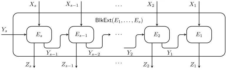
Definition 2.0.11 (block source extraction by composition). Let s ≥ 1 be an integer and for each i ∈ [s], let Ei : Fnqi ×Fdqi → Fmqi be a map. Suppose that mi ≥ di−1 for all i∈ [s],

where we define d0 = 0. DefineE =BlkExt(E1, . . . , Es) as follows:

E : (_Fn1

q × · · · ×F ns

q )×F ds

q →(F m1−d0

q × · · · ×F

ms−ds−1

q )

((x1, . . . , xs), ys)7→(z1, . . . , zs)

where for i =s, . . . ,1, we iteratively define (yi−1, zi) to be a partition of Ei(xi, yi) into the

prefix yi−1 ∈F

di−1

q and the suffix zi ∈F mi−di−1

q .

See Figure 2.1 for an illustration of the above definition.

Lemma 2.0.9. Let s ≥ 1 be an integer and for each i ∈ [s], let Ei : Fqni ×Fdqi → Fmqi be

a (ki, i, q) extractor of degree ti ≥ 1. Then E = BlkExt(E1, . . . , Es) is a ((k1, . . . , ks), , q)

block source extractor of degree t where =Ps

i=1i and t=

Qs

i=1ti.

Proof. Induct ons. When s= 1 the claim follows from the extractor property of E1.

When s > 1, assume the claim holds for all s0 < s. Define E0 =BlkExt(E2, . . . , Es). By

the induction hypothesis,E0 is a ((k2, . . . , ks), 0, q) block source extractor where0 =

Ps i=2i

and t0 =Qs

Es Es−1 · · ·

· · ·

· · ·

E2 E1

Ys

Xs Xs−1 X2 X1

Zs Zs−1 Z2 Z1

Ys−1 Ys−2 Y2 Y1

BlkExt(E1, . . . , Es)

Figure 2.1: The composed block source extractorBlkExt(E1, . . . , Es)

Let (X1, . . . , Xs) ⊂ Fnq1 × · · · ×Fnqs be an arbitrary (k1, . . . , ks) q-ary block source. Let

(Yi−1, Zi) ⊂ F di−1

q × Fqmi−di−1 be the output of Ei and (Z1, . . . , Zs) be the the output of

E when (X1, . . . , Xs) is fed into E as the input and an independent uniform distribution

Ys =Uds,q is used as the seed (c.f. Figure 2.1). The output of E

0 _{is then (Y}

1, Z2, . . . , Zs).

Fix x∈supp(X1). By the definition of block sources, the distribution (X2, . . . , Xs)|X1=x

is a (k2, . . . , ks) q-ary block source. Also note that Ys|X1=s =Ys is an independent uniform

distribution. By the induction hypothesis, the distribution

(Y1, Z2, . . . , Zs)|X1=x =E 0

((X2, . . . , Xs), Ys)|X1=x

is0-close to (Ud1,q, Um2−d1,q, . . . , Ums−ds−1,q). As this holds for allx∈supp(X1), the

distribu-tion (X1, Y1, Z2, . . . , Zs) is0-close to (X1, Ud1,q, Um2−d1,q, . . . , Ums−ds−1,q). So the distribution

E((X1, . . . , Xs), Ys) = (E1(X1, Y1), Z2, . . . , Zs)

is0-close to (E1(X1, Ud1,q), Um2−d1,q, . . . , Ums−ds−1,q). Then we know that it is also -close to

(Um1−d0,q, Um2−d1,q, . . . , Ums−ds−1,q) since E1 is a (k1, 1, q) extractor.

Finally, to see that E has degree t, note that E0((X2, . . . , Xs), Ys) = (Y1, Z2, . . . , Zs)

has degree t0 in its variables X2, . . . , Xs and Ys by the induction hypothesis and hence

Y1, Z2, . . . , Zs have degree t0 in these variables. Then Z1 = E1(X1, Y1) has degree t1 ·

max{1, t0} = t in X1, . . . , Xs and Ys. So E((X1, . . . , Xs), Ys) = (Z1, . . . , Zs) has degree t

Chapter 3

Basic results

3.1

Extractor vs. sampler connection

Our construction of curve samplers relies on the following observation by [Zuc97] which shows the equivalence between extractors and samplers.

Theorem 3.1.1 ([Zuc97], restated). Given a map f :_Fn_q×_Fd

q →Fmq , we have the following:

(1) If f is a (k, , q) extractor, then it is also an (, δ) sampler where δ= 2qk−n. (2) If f is an (/2, δ) sampler where δ =qk−n, then it is also a (k, , q) extractor.

Proof. (Extractor to sampler) Assume to the contrary thatf is not an (, δ) sampler. Then there exists a subsetA⊆_Fm

q with Prx[|µf(x)(A)−µ(A)|> ]> δ. Then either Prx[µf(x)(A)−

µ(A)> ]> δ/2 or Prx[µf(x)(A)−µ(A)<−]> δ/2. Assume Prx[µf(x)(A)−µ(A)> ]> δ/2

(the other case is symmetric). LetX be the uniform distribution over the set ofx such that µf(x)(A)−µ(A)> , i.e., Pry[f(x, y)∈ A]−Prx[x ∈ A] > . Then |f(X, Ud,q)−Um,q| > .

But the q-ary min-entropy of X is at least log_q((δ/2)qn_{) ≥ k, contradicting the extractor}

property of f.

(Sampler to extractor) Assume to the contrary that f is not a (k, , q) extractor. Then there exists a subset A⊆_Fm

q and a random source X of q-ary min-entropy k satisfying the

property that |Pr[f(X, Ud,q) ∈ A]−µ(A)| > . We may assume X is a flat source (i.e.

uniformly distributed over its support) since a general source with q-ary min-entropy k is a convex combination of flat sources with q-ary min-entropy k. Note that|supp(X)| ≥qk_{. By}

the averaging argument, for at least an -fraction of x∈ supp(X), we have|Pr[f(x, Ud,q)∈

A]−µ(A)| > /2. But it implies that for x uniformly chosen from _Fn

q, with probability at

leastµ(supp(X)) =δ we have|µf(x)(A)−µ(A)|> /2, contradicting the sampling property

Table 3.1 shows the rough correspondences between the parameters of extractors and those of samplers.

extractor sampler

error accuracy error

entropy deficiency (n−k) logq confidence error δ seed length dlogq sample complexity qd

input lengthnlogq randomness complexity nlogq output length mlogq domain sizeqm

Table 3.1: The correspondences between the parameters of extractors and samplers

3.2

Existence of a good curve sampler

In this section, we prove the existence of a (non-explicit) low-degree curve sampler with low randomness complexity and a small number of sample points.

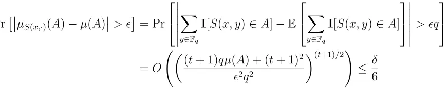
Theorem 3.2.1. For any m ≥ 1, , δ > 0 and sufficiently large q ≥ log(1/δ)Θ(1), there exists a (non-explicit) (, δ) degree-t curve sampler S : D × _Fq → Fmq with randomness

complexity log|D| =mlogq+ log (1/δ) +O(1), sample complexity q, and t=O log_q(1/δ). Proof. We use the probabilistic method. Choose the curve samplerS by choosing the degree-t curve S(x,·) :_Fq →Fmq independently at random for each x∈ D.

Let A be an arbitrary subset of _Fm

q . Fix x ∈ D. By Lemma 2.0.2, the random

vari-ables S(x, y) with y ranging over _Fq are (t + 1)-wise independent. So the indicator

vari-ables I[S(x, y) ∈ A] with y ranging over _Fq are also (t + 1)-wise independent. Applying

Lemma 2.0.5, we get

PrµS(x,·)(A)−µ(A)

> = Pr   X

y∈Fq

I[S(x, y)∈A]−_E



 X

y∈Fq

I[S(x, y)∈A]   > q   =O

(t+ 1)qµ(A) + (t+ 1)2

2_q2

(t+1)/2!

≤ δ

6

for sufficiently large β. Let B(x) be the event that µS(x,·)(A)−µ(A)

> . Then 0 ≤ Pr [I[B(x)] = 1] ≤ δ

6 and hence E[

P

xI[B(x)]] ≤ δ|D|

6 . The indicator variables I[B(x)] with

x ranging over D are independent. Applying Lemma 2.0.3, we obtain

Pr "

X

I[B(x)]≥δ|D|

#

There are 2qm

possibleA⊆_Fm

q . So with probability at least 1−2q

m

2−δ|D|_{>0 (for sufficiently}

large log|D| =mlogq+log (1/δ)+O(1)), the eventsP

xI[B(x)]≤δ|D|for allA⊆F m q occur

by the union bound. Take the curve sampler S that makes all these events occur. Then S is an (, δ) degree-t curve sampler by definition.

The most interesting case is when the domain size qm and the confidence error δ are polynomially related, while the field size q and the degree t are kept small:

Corollary 3.2.1. Given the domain size N = |_Fm

q |= qm, accuracy error = (logN)

−O(1)

, confidence error δ = N−O(1)_{, and large enough field size q = (logN)}Θ(1)

, there exists a (non-explicit) (, δ) degree-t curve sampler S : D ×_Fq → Fmq with randomness complexity

log|D|=O(logN), sample complexity q, and t= Θ_{log log}logN_N.

3.3

Lower bounds

We will use the following optimal lower bound for extractors:

Theorem 3.3.1 ([RTS00], restated). Let E :_Fn_q ×_Fd

q →Fmq be a (k, , q) extractor. Then

(a) if <1/2 and qd_≤qm_{/2, then q}d _{= Ω}(n−k) logq 2

, and (b) if qd_≤qm_{/4, then q}d+k−m _{= Ω(1/}2_).

Theorem 3.3.2. Let S:_Fn

q×Fq→Fmq be an (, δ)curve sampler where <1/2and m≥2.

Then

(a) the sample complexity q= Ωlog(22/δ)

, and

(b) the randomness complexity nlogq≥(m−1) logq+ log(1/) + log(1/δ)−O(1).

Proof. By Theorem 3.1.1,Sis a (k,2, q) extractor wherek =n−log_q(2/δ). The first claim then follows from Theorem 3.3.1 (a). Applying Theorem 3.3.1 (b), we get (1 +k−m) logq≥

Ω(log(1/))−O(1). Therefore

nlogq =klogq+ log(2/δ)≥(m−1) logq+ log(1/δ) + Ω(log(1/))−O(1).

In particular, as log(1/) = O(logq), the randomness complexity nlogq is at least Ω(logN + log(1/δ)) when the domain size N = qm ≥ N0 for some constant N0.

There-fore the randomness complexity in Theorem 1.0.1 is optimal up to a constant factor.

Theorem 3.3.3. Let S : N ×_Fq → Fmq be an (, δ) degree-t curve sampler where m ≥ 2,

<1/2 and δ <1. Then t = Ω log_q(1/δ) + 1 .

Proof. Clearly t ≥1. Suppose S = (S1, . . . , Sm) and define S0 = (S1, S2). LetC be the set

of curves of degree at most t in _F2

q. Then |C| = q2(t+1). Consider the map τ : N → C that

sendsxtoS0(x,·). We can pick k=bq/2ccurvesC1, . . . , Ck ∈ C such that the union of their

preimages

B def=

k

[

i=1

τ−1(Ci) = k

[

i=1

{x:S0(x,·) = Ci}

has size at least k_|C||N | = _q2(k|N |t+1).

Define A⊆_Fm q by

Adef={Ci(y) :i∈[k], y ∈Fq} ×Fmq −2,

i.e., let A be the set of points in _Fm

q whose first two coordinates are on at least one curve

Ci. We have |A| ≤ kqm−1 and hence µ(A) ≤ k/q ≤ 1/2 < 1−. On the other hand, it

follows from the definition of A that we have S(x, y) ∈ A for all x ∈ B and y ∈ _Fq. So

µS(x)(A) = 1 for all x ∈ B. Then δ ≥ Pr

|µS(x)(A)−µ(A)|>

≥ _{|N |}|B| ≥ k

q2(t+1) and hence

t≥max1,1₂log_q(k/δ)−1 = Ω log_q(1/δ) + 1.

Chapter 4

Explicit constructions

4.1

Outer sampler

In this section we construct an O(logk)-dimensional manifold sampler, which we called the “outer sampler”, with the optimal randomness complexity where k = n −log_q(1/δ). In the language of extractors, we construct an extractor with the seed in _FOq(logk) for random

sources of q-ary min-entropy k.

4.1.1

Block source conversion

Definition 4.1.1(block source converter [NZ96]).A functionC :_Fn

q×Fdq →(Fqm1×· · ·×Fmqs)

is called a (k,(k1, . . . , ks), , q) block source converter if for any random source X ⊆ Fnq of

q-ary min-entropyk, the outputC(X, Ud,q)⊂Fmq1× · · · ×Fmqs is-close to a (k1, . . . , ks)q-ary

block source. In addition, we say C has degree t if C has degree t as a manifold in _Fn+d q .

It was shown in [NZ96] that one can obtain a block by choosing a pseudorandom subset of bits of the random source. Yet the proof is pretty delicate and cumbersome. Furthermore the resulting extractor does not have a nice algebraic structure. Here we make the observation that the following condenser from Reed-Solomon codes in [GUV09] can be used to obtain blocks and is a low-degree manifold.

Definition 4.1.2(condenser from Reed-Solomon codes [GUV09]). Letζ ∈_Fqbe a generator

of the multiplicative group _F×_q. Define RSConn,m,q : Fnq ×Fq →Fmq for n, m ≥1 and prime

power q:

RSConn,m,q(x, y) = y, fx(y), fx(ζy), . . . , fx(ζm−2y)

where fx(Y) = Pn

−1

i=0 xiY

i _{for x= (x}

Theorem 4.1.1 ([GUV09]). For any h ≥ 1, n ≥ m ≥ 1, prime power q and > 0, RSConn,m,q is an n,logq

H

→2,q m,logq L

2

condenser, where H = (h−1)qm_q−₋1₁−1 and L = (q−(n−1)(h−1)(m−1))·hm−1 _{−1. In particular, for large enough q ≥ (n/)}O(1)_,

RSConn,m,q is a m →,q 0.99m condenser.

Remark 3. The condenser RSConn,m,q(x, y) is a degree-n manifold, as each monomial in any

of its coordinate is of the form y or xi(ζjy)i where i≤n−1.

Remark 4. The reason we use the condenser from Reed-Solomon codes rather than the ones from Parvaresh-Vardy codes [GUV09, TSU12] is that we need the condenser to be a low-degree manifold in both the seed and the random source. The known condensers from Parvaresh-Vardy codes are low-degree in the seed, yet we have no good bound on the degree in the random source.

We apply the above condenser on the random source with an independent seed to obtain a new block each time. Formally:

Definition 4.1.3 (block source converter via condensing). For integers n, m1, . . . , ms ≥ 1

and prime power q, define the functionBlkCnvtn,(m1,...,ms),q :F

n

q ×Fsq →Fm1+

···+ms

q by

BlkCnvtn,(m1,...,ms),q(x, y) = (RSConn,m1,q(x, y1), . . . ,RSConn,ms,q(x, ys))

for x∈_Fn

q and y= (y1, . . . , ys)∈Fsq.

The function BlkCnvtn,(m1,...,ms),q is indeed a block source converter, as we show below.

The intuition is that conditioning on the values of the previous blocks, the random sourceX still has enough min-entropy, and hence we may apply the condenser to get the next block.

We need the following technical lemmas:

Lemma 4.1.1. Let P, Q⊂I be two distributions with ∆(P, Q)≤. Let {Xi :i∈supp(P)}

and {Yi : i ∈ supp(Q)} be two collections of distributions over the same domain S such

that ∆(Xi, Yi)≤ 0 for any i ∈ supp(P)∩supp(Q). Then X

def

=P

i∈supp(P)Pr[P =i]·Xi is

(2+0)-close to Y def=P

i∈supp(Q)Pr[Q=i]·Yi.

Proof. LetT be an arbitrary subset of S and we will prove that|Pr[X ∈T]−Pr[Y ∈T]| ≤

2+0.

Note that we can add dummy distributions Xi for i ∈ I \supp(P) and Yj for j ∈

I\supp(Q) such that ∆(Xi, Yi)≤0for alli∈I, and it still holds thatX =

P

and Y =P

i∈IPr[Q=i]·Yi. Then we have

|Pr[X ∈T]−Pr[Y ∈T]|

= X

i∈I

Pr[P =i] Pr[Xi ∈T]−

X

i∈I

Pr[Q=i] Pr[Yi ∈T]

≤X

i∈I

|Pr[P =i] Pr[Xi ∈T]−Pr[Q=i] Pr[Yi ∈T]|

≤X

i∈I

|(Pr[P =i]−Pr[Q=i]) Pr[Xi ∈T] + Pr[Q=i](Pr[Xi ∈T]−Pr[Yi ∈T])|

≤ X

i∈I

|Pr[P =i]−Pr[Q=i]|

!

+0 X

i∈I

Pr[Q=i] !

≤2+0

Lemma 4.1.2. LetX = (X1, . . . , Xs)⊂Fqn1×· · ·×Fnqs be a distribution such that for anyi∈

[s] and (x1, . . . , xi−1)∈supp(X1, . . . , Xi−1), the conditional distribution Xi|X1=x1,...,Xi−1=xi−1

is -close to a distribution X˜i(x1, . . . , xi−1) with q-ary min-entropy ki. Then X is 2s-close

to a (k1, . . . , ks) q-ary block source.

Proof. DefineX0 = (X₁0, . . . , X_s0) as the unique distribution such that for any i∈[s] and any (x1, . . . , xi−1)∈supp(X10, . . . , X

0

i−1), the conditional distribution X

0

i|X0

1=x1,...,X_i0−1=xi−1 equals

˜

Xi(x1, . . . , xi−1) if (x1, . . . , xi−1)∈supp(X1, . . . , Xi−1)1 and otherwise equalsUni,q.

For any i ∈ [s] and (x1, . . . , xi−1) ∈ supp(X10, . . . , X

0

i−1), we known X

0

i|X0

1=x1,...,X0i−1=xi−1

is either ˜Xi(x1, . . . , xi−1) or Uni,q. And in either case it has min-entropy ki. So X

0 _{is a}

(k1, . . . , ks) q-ary block source.

We will then prove that for any i ∈ [s] and any (x1, . . . , xi−1) ∈ supp(X1, . . . , Xi−1)∩

supp(X₁0, . . . , X_i0₋₁), the conditional distribution X|X1=x1,...,Xi−1=xi−1 is 2(s−i+ 1)-close to

X0|X₁0=x1,...,Xi0−1=xi−1. Setting i= 1 proves the lemma.

Induct on i. For i = s the claim holds by the definition of X0. For i < s, assume the claim holds for i + 1 and we will prove that it holds for i as well. Consider any (x1, . . . , xi−1)∈supp(X1, . . . , Xi−1)∩supp(X10, . . . , Xi0−1). LetA =Xi|X1=x1,...,Xi−1=xi−1 and

B =X_i0|_X0

1=x1,...,X_i0−1=xi−1. We have

X|X1=x1,...,Xi−1=xi−1 =

X

xi∈supp(A)

Pr[A =xi]·X|X1=x1,...,Xi=xi

1_(x

and

X0|X0

1=x1,...,X_i0−1=xi−1 =

X

xi∈supp(B)

Pr[B =xi]·X0|X0

1=x1,...,X0_i=xi.

By the induction hypothesis, we have

∆ X|X1=x1,...,Xi=xi, X

0_|

X₁0=x1,...,X_i0=xi

≤2(s−i)

for xi ∈ supp(A)∩supp(B). Also note that B is identical to ˜Xi(x1, . . . , xi−1) and is -close

toA by definition. The claim then follows from Lemma 4.1.1. Now we are ready to prove the following theorem.

Theorem 4.1.2. For >0, integers s, n, m1, . . . , ms≥1 and sufficiently large prime power

q = (n/)O(1)_{, the function BlkCnvt}

n,(m1,...,ms),q is a (k,(k1, . . . , ks),3s, q) block source

con-verter of degree n where k =Ps

i=1mi+ logq(1/) and each ki = 0.99mi.

Proof. The degree of BlkCnvtn,(m1,...,ms),q is n since RSConn,m,q has degree n. Let X be a

random source that has q-ary min-entropy k. Let Y1, . . . , Ys be independent seeds uniformly

distributed over _Fq. Let Z = (Z1, . . . , Zs) = BlkCnvtn,(m1,...,ms),q(X,(Y1, . . . , Ys)) where each

Zi =RSConn,mi,q(X, Yi) is distributed over F

mi

q . Define

B = (

(z1, . . . , zi) :

i∈[s], (z1, . . . , zi)∈supp(Z1, . . . , Zi), X|Z1=z1,...,Zi=zi does not

have q-ary min-entropy k−(m1+· · ·+mi)−logq(1/)

) .

Define a new distribution Z0 = (Z₁0, . . . , Z_s0) as follows: Samplez = (z1, . . . , zs)←Z and

independentlyu= (u1, . . . , us)←Um1+...,+ms,q. If there existi∈[s] such that (z1, . . . , zi−1)∈

B, then pick the smallest such i and let z0 = (z1, . . . , zi−1, ui, . . . , us). Otherwise let z0 =z.

LetZ0 be the distribution of z0.

For any i ∈[s] and (z1, . . . , zi−1)∈ supp(Z10, . . . , Zi0), if some prefix of (z1, . . . , zi−1) is in

B then Z_i0|Z₁0=z1,...,Zi0−1=zi−1 is the uniform distribution Umi,q, otherwise Z

0

i|Z₁0=z1,...,Zi0−1=zi−1 =

Zi|Z1=z1,...,Zi−1=zi−1. In the second case, X|Z1=z1,...,Zi−1=zi−1 has min-entropy k−(m1+· · ·+

mi−1)−logq(1/)≥mi since (z1, . . . , zi−1)6∈B. In this case, Zi0|Z₁0=z1,...,Z_i0−1=zi−1 is -close to

a distribution of min-entropy ki by Theorem 4.1.1 and the fact

Z_i0|Z0

1=z1,...,Z0i−1=zi−1 =Zi|Z1=z1,...,Zi−1=zi−1 =RSConn,mi,q(X|Z1=z1,...,Zi−1=zi−1, Yi).

In either cases Z_i0|Z₁0=z1,...,Z_i0−1=zi−1 is -close to a distribution of min-entropy ki. By

Lemma 4.1.2,Z0 is 2s-close to a (k1, . . . , ks)q-ary block source.

B] ≤ . So the probability that (Z1, . . . , Zi−1) ∈ B for some i ∈ [s] is bounded by s.

Note that the distributionZ0 is obtained fromZ by redistributing the weights of (z1, . . . , zs)

satisfying (z1, . . . , zi−1)∈B for some i. We conclude that ∆(Z, Z0)≤s, as desired.

4.1.2

Block source extraction

We will employ Lemma 2.0.9 and compose some “basic” extractors to get a block source extractor. These basic extractors are given by the basic line samplers Linem,q (see

Defini-tion 2.0.4).

Lemma 4.1.3. For >0, m≥1 and prime powerq, Linem,q is a (k, , q)extractor of degree

2 where k= 2m−1 + 3 log_q(1/).

Proof. Apply Lemma 2.0.6 and Theorem 3.1.1.

Suppose _FQ is an extension field ofFq with [FQ :Fq] =d, i.e., Q=qd. By Lemma 2.0.1,

Linem,Q :F2Qm×FQ →FmQ, as a degree-2 manifold overFQ, can also be viewed as a degree-2

manifold over _Fq: Linem,Q :Fq2md×Fdq →Fmdq .

Now we are ready to state the main result of this section. We first compose the basic line samplers to get a block source extractor. It is then applied to a block source obtained from the block source converter.

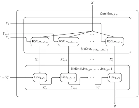
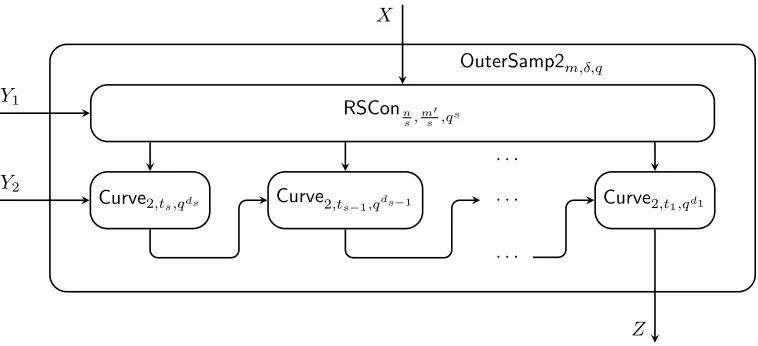
Definition 4.1.4 (Outer Sampler). For δ > 0, m = 2s _{and prime power q, let n = 4m+}

log_q(2/δ),d =s+ 1, anddi = 2s−i for i∈[s]. Fori∈[s], viewLine2,qdi :F4_qdi×Fqdi →F2_qdi

as a manifold over _Fq: Line2,qdi :F4di

q ×Fdqi →Fq2di. Composing these line samplers Line2,qdi

for i∈ [s] gives the functionBlkExt(Line_2,qd₁, . . . ,Line_2,qds) : _Fq4d1+···+4ds ×_Fq →_Fm_q . Finally,

define OuterSamp_m,δ,q :_Fn_q ×_Fd

q →Fmq :

OuterSamp_m,δ,q(x,(y, y0))def=BlkExt(Line_2,qd1, . . . ,Line2,qds) BlkCnvtn,(4d1,...,4ds),q(x, y), y

0

for x∈_Fn

q, y∈Fsq and y

0 _∈

Fq.

See Figure 4.1 for an illustration of the above definition.

Theorem 4.1.3. For any , δ > 0, integer m ≥ 1, and sufficiently large prime power q ≥ (n/)O(1), OuterSamp_m,δ,q is an (, δ) sampler of degree t where d = O(logm), n = O m+ log_q(1/δ)

and t=O m2_+mlog

q(1/δ)

.

Proof. We first show that OuterSamp_m,δ,q is a (4m, , q) extractor. Consider any random source X over _Fn

q with q-ary min-entropy 4m. Let s, di be as in Definition 4.1.4. Let

RSConn,ds,q RSConn,ds−1,q · · ·

· · ·

RSConn,d1,q X

Ys

Ys−1

.. .

Y1

BlkCnvtn,(4d1,...,4ds),q

Line2,qds Line_2,qds−1 · · · Line2,qd1

· · ·

Xs0 Xs0−1 X10

Y0 =Y_s0

Z

Y_s0₋₁ Y_s0₋₂ Y₁0

BlkExt Line2,qd1, . . . ,Line2,qds OuterExtn,k,q

Figure 4.1: The extractor OuterExtn,k,q that takes the random source X together with the

seed (Y1, . . . , Ys, Y0) and then outputs Z.

We have (Ps

i=14di) + logq(1/0)≤ 4m for sufficiently large q ≥ (n/)O(1). So by

Theo-rem 4.1.2,BlkCnvtn,(4d1,...,4ds),qis a (4m,(k1, . . . , ks),3s0, q) block source converter. Therefore

the distributionBlkCnvtn,(4d1,...,4ds),q(X, Us,q) is 3s0-close to a (k1, . . . , ks)q-ary block source

X0. Then OuterSamp_m,δ,q(X, Ud,q) is 3s0-close to BlkExt(Line2,qd₁, . . . ,Line_2,qds)(X0, U_1,q).

By Lemma 4.1.3,Line_2,qdi is a ki/di, 0, qdi

extractor fori∈[s] since 3 + 3 log_qdi(1/0)≤

4·0.99 = ki/di. Equivalently it is a (ki, 0, q) extractor.

By Lemma 2.0.9, BlkExt(Line_2,qd₁, . . . ,Line_2,qds) is a ((k₁, . . . , k_s), s₀, q) block source

ex-tractor. Therefore BlkExt(Line_2,qd₁, . . . ,Line_2,qds)(X0, U_1,q) is s₀-close to U_m,q, which by the

previous paragraph, implies thatOuterSamp_m,δ,q(X, Ud,q) is 4s0-close toUm,q. By definition,

OuterSamp_m,δ,q is a (4m, , q) extractor. By Theorem 3.1.1, it is also an (, δ) sampler. We haved=s+1 =O(logm) andn =O m+ log_q(1/δ)

. By Lemma 2.0.1, eachLine_2,qdi

has degree 2s_{. By Theorem 4.1.2,BlkCnvt}

n,(4d1,...,4ds),q has degreen. ThereforeOuterSampm,δ,q

has degree n2s _{=O m}2_+mlog

q(1/δ)

.

Remark 5. We assume mis a power of 2 above. For generalm, simply pickm0 = 2dlogme and let OuterSamp_m,δ,q be the composition of OuterSamp_m0_,δ,q with the projection π :_Fm

0

q →Fmq

onto the first m coordinates. It yields an (, δ) sampler of degree t for _Fm_q since π is linear, and approximating the density of a subsetAin_Fm_q is equivalent to approximating the density of π−1_{(A) in}

Fm

0 q .

Remark 6. The most important properties of the extractorsLine_2,qdi used here are (1) they

work for a certain constant min-entropy rate, and (2) the seed is shorter than the output by a constant factor. As the reader can check, besides the basic line samplers, we may also use the randomness-efficient line samplers given by [MR06], or the (strong) extractors from the universal family of hash functions {ha,b :x7→ax+b} [CW79] (operations are performed in

a finite field) together with the leftover hash lemma [ILL89], etc.

The sampler OuterSamp_m,δ,q has optimal randomness complexity O(mlogq+ log (1/δ)), yet the sample complexity is sub-optimal, being qd =qO(logm) instead of q. We will fix this problem by composing it with an “inner sampler” that has the optimal sample complexity.

4.2

Inner sampler

We will construct a curve sampler of low degree in this section, or what we called the “inner sampler”. It might be viewed as an extractor with optimal seed length, even though it only extracts a tiny fraction of min-entropy from the random source. The construction will be based on two techniques called error reduction and iterated sampling.

4.2.1

Error reduction

Condensers are at the core of many extractor constructions [RSW06, TSUZ07, GUV09, TSU12]. In the language of samplers, the use of condensers can be regarded as an error reduction technique, as we shall see below.

Given a functionf :_Fn

q×Fdq →Fmq , define LISTf(T, )

def

=x∈_Fn

q : Pry[f(x, y)∈T]>

for anyT ⊆_Fm

q and >0. We are interesting in functionsf exhibiting a “list-recoverability”

property that the size of LISTf(T, ) is kept small when T is not too large.

Definition 4.2.1. A functionf :_Fn

q×Fq →Fmq is (, L, H)list-recoverableif|LISTf(T, )| ≤

H for all T ⊆_Fm

Remark 7. The above definition is justified as an extension oflist-recoverable codes[GI01]: A codeC ⊆_Fn

q is called (ρ, L, H) list recoverableif for any setsS1, . . . , Sn ⊆Fq of size at most

L, there are at mostHcodewordsx= (x1, . . . , xn)∈Csuch that Pri∈[n][xi ∈Si]>1−ρ. Let

f :_Fn

q ×Fq →Fmq be an (, H, L) list-recoverable function. Assume f = (f1, . . . , fm) has the

extra property that f1(x, y) =y for all x∈Fnq and y∈Fq (in particular, the Reed-Solomon

condenser in Definition 4.1.2 has this property). Define code Cf ⊆ Fmq−1

q

as follows:

Cf =

(f2(x, y1), . . . , fm(x, yq)) :x∈Fnq

wherey1, . . . , yqare theqdistinct elements ofFq(in any order). ThenCf is (1−, H, L/q)

list-recoverable: For anyS1, . . . , Sq⊆Fmq −1 of size at mostL/q, letT =

Sq

i=1({yi} ×Si)⊆Fmq be

their union that has size at most L. By definition, every codeword (f2(x, y1), . . . , fm(x, yq))

satisfying Pri∈[n][xi ∈ Si] > corresponds to an element x ∈ |LISTf(T, )|. Therefore the

number of such codewords is upper bounded by|LISTf(T, )| ≤H.

The following lemma shows that the condenser property implies the list-recoverability property.

Lemma 4.2.1 ([GUV09]). Suppose f : _Fn

q ×Fdq → Fmq is an (n,logqH) →,q m,logq L

condenser. Then it holds that |LISTf(T,2)| ≤ H for any T ⊆ Fmq of size at most L, and

hence f is (2, L, H) list-recoverable.

We then define an operation ? as follows.

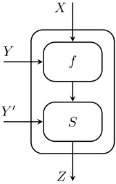
Definition 4.2.2. For functions f : _Fn_q × _Fd

q → Fmq and S : Fmq × Fd 0

q → Fm 0

q , define

S ? f :_Fn

q ×(Fdq×Fd 0

q )→Fm 0

q as follows:

S ? f(x,(y, y0))def=S(f(x, y), y0). See Figure 4.2 for an illustration of the above definition.

The following lemma states that a sampler with mildly small confidence error, when composed with a list-recoverable function via the ? operation, gives a sampler with very small confidence error.

Lemma 4.2.2. Supposef :_Fn

q ×Fdq →Fmq is (1, L, H) list-recoverable, and S :Fmq ×Fd 0

q →

Fm

0

q is an (2, δ) sampler where δ= _qLm. Then S ? f is an

1 +2,_qHn

sampler.

Proof. Let A be an arbitrary subset of _Fm0

q . Let B = {y : |µS(y,·) −µ(A)| > 2}. By the

sampler property of S, we have |B| ≤δqm =L and hence |LISTf(B, 1)| ≤ H. Therefore it

suffices to show that for anyx∈_Fn

f

S X

Y

Y0

Z

Figure 4.2: The function S ? f. The output is denoted by Z. Fix x∈_Fn

q \LISTf(B, 1). We have

µS?f(x,·)(A) = Pr

y,y0[S ? f(x,(y, y

0

))∈A] = Pr

y,y0[S(f(x, y), y

0

)∈A] =_Ey

µS(f(x,y),·)(A)

.

Therefore

|µS?f(x,·)(A)−µ(A)|=

E_y

µS(f(x,y),·)(A)

−µ(A)

≤_Ey|µS(f(x,y),·)(A)−µ(A)|

≤Pr

y [f(x, y)∈B] +2Pry [f(x, y)6∈B]

≤1+2.

To see the last two steps, note that |µS(y,·)(A)−µ(A)| ≤ 2 for y 6∈ B by definition, and

Pry[f(x, y)∈B]≤1 since x6∈LISTf(B, 1).

Combining Lemma 4.2.1 and Lemma 4.2.2, we obtain:

Corollary 4.2.1. Suppose f : _Fn_q ×_Fd

q → Fmq is an (n, k1) →,q (m, k2) condenser, and

S :_Fm q ×Fd

0

q →Fm 0

q is an

0_{, q}k2−m _{sampler. Then S ? f is an 2+}0_{, q}k1−n _sampler.

Proof. Lemma 4.2.1 implies |LISTf(T,2)| ≤ qk1 for T of size at most qk2. Set H = qk1,

L=qk2_,

1 = 2, 2 =0 and apply Lemma 4.2.2.

Remark 8. It also possible to prove Corollary 4.2.1 using the connection between extractors and samplers (c.f. Theorem 3.1.1), except that some parameters are slightly different, e.g. the resulting accuracy error is+20 which has poorer dependence on0, due to the averaging argument used in the proof of Theorem 3.1.1.

[GUV09, TSU12], not the other way around. So we choose to use the list-recoverability properties directly, together with Lemma 4.2.2.

The condenser RSConn,m,q from Reed-Solomon codes (see Definition 4.1.2) enjoys the

following list-recoverability property:

Theorem 4.2.1 ([GUV09]). For any h ≥ 1, n ≥ m ≥ 1, prime power q and > 0, RSConn,m,q is (, L, H) list-recoverable where H = (h−1)q

m−1₋₁

q−1 and L= (q−(n−1)(h−

1)(m − 1)) ·hm−1 _{− 1. In pariticular, for sufficiently large q ≥ (n/)}O(1)_{, RSCon}

n,m,q is

(, q0.99m_{, q}m_{) list-recoverable.}

Corollary 4.2.2. For any n ≥ m ≥ 1, , 0 > 0 and sufficiently large prime power q = (n/)O(1), supposeS:_Fm_q ×_Fd

q →Fm 0

q is an(0, q−0.01m)sampler of degreet, thenS?RSConn,m,q

is an (+0, qm−n) sampler of degree nt.

Proof. Apply Lemma 4.2.2 and Theorem 4.2.1. Note that RSConn,m,q has degree n.

There-fore (S ?RSConn,m,q) (X,(Y, Y0)) = S(RSConn,m,q(X, Y), Y0) has degree nt in its variables

X, Y, Y0.

4.2.2

Iterated sampling

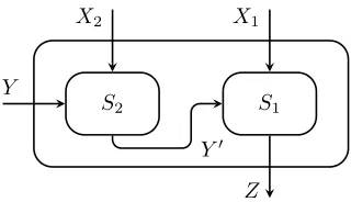
We introduce the operation ◦ performed on samplers.

Definition 4.2.3. (composed sampler). Given functions S1 : Fnq1 × Fqd1 → Fdq0 and S2 :

Fn2

q ×Fdq2 →Fqd1, define S1◦S2 : (Fqn1 ×Fnq2)×Fqd2 →Fdq0 such that

S1◦S2((x1, x2), y)

def

=S1(x1, S2(x2, y))

for all x1 ∈Fnq1, x2 ∈Fnq2 and y∈Fdq2.

See Figure 4.3 for an illustration of the above definition.

S2 S1

Y

X2 X1

Z Y0

Figure 4.3: The function S1◦S2. The output is denoted byZ.

Think of S1 and S2 as samplers. Then S1 ◦S2 is the composed sampler that first uses

subsample S2(x1, S2(x2,·))⊆S1(x1,·). Intuitively, if S1 and S2 are good samplers then so is

S1◦S2. This is indeed shown by [BR94, TSU06] and we formalize it as follows:

Lemma 4.2.3. Let S1 : Fnq1 ×Fdq1 → Fdq0 be an (1, δ1) manifold sampler of degree t1.

And let S2 : Fnq2 ×Fdq2 → Fqd1 be an (2, δ2) manifold sampler of degree t2. Then S1 ◦S2 :

(_Fn1

q ×Fnq2)×Fdq2 →Fdq0 is an (1+2, δ1+δ2) manifold sampler of degree t1t2.

Proof. Consider an arbitrary subset A ⊆ _Fd0

q . Define B(x) =

z ∈_Fd2

q :S1(x, z)∈A for

each x ∈ _Fn1

q . Pick x1 ← Un1,q and x2 ← Un2,q. If

µS1◦S2((x1,x2),·)(A)−µ(A)

> ₁ +₂ occurs, then either|µS1(x1,·)(A)−µ(A)|> 1, or|µS1◦S2((x1,x2),·)(A)−µS1(x1,·)(A)|> 2 occurs.

Call the two events E1 and E2 respectively.

Note that E1 occurs with probability at most δ1 by the sampler property of S1. Also

note that

µS1◦S2((x1,x2),·)(A) = Pr

y [S1(x1, S2(x2, y))∈A] = Pry [S2(x2, y)∈B(x1)] = µS2(x2,·)(B(x1))

whereas

µS1(x1,·)(A) = Pr

y [S1(x1, y)∈A] = Pry [y∈B(x1)] = µ(B(x1)).

So the probability that E2 occurs is Prx1,x2[|µS2(x2,·)(B(x1)) − µ(B(x1))| > 2] which is

bounded by δ2 by the sampler property of S2. By the union bound, the event

µS1◦S2((x1,x2),·)(A)−µ(A)

> ₁+₂ occurs with probability at mostδ1+δ2, as desired.

Finally, we have S1◦S2((X1, X2), Y)) = S1(X1, S2(X2, Y)) which is a manifold of degree

t1t2 in its variablesX1, X2, Y since S1 and S2 are manifolds of degree t1 and t2 respectively.

A simple induction implies the following generalization of Lemma 4.2.3:

Corollary 4.2.3. Let Si :Fnqi×Fdqi →F di−1

q be an (i, δi)sampler that is a manifold of degree

ti fori= 1, . . . , s. ThenS1◦ · · · ◦Ss : Fnq1 × · · · ×Fnqs

×_Fds

q →Fdq02 is an(

Ps

i=1i,

Ps

i=1δi)

sampler that is a manifold of degree Qs

i=1ti.

Remark 9. The readers may notice that the composed sampler S1 ◦S2 has the same form

as the composed block source extractor BlkExt(S1, S2) (see Definition 2.0.11), and more

generally S1 ◦ · · · ◦Ss has the same form as BlkExt(S1, . . . , Ss) (with the outputs Zs, . . . , Z2

being empty strings, c.f. Figure 2.1). This is not a coincidence. Using the connection between

2_{It is easy to check that◦is associative, and hence we can writeS}

extractors and samplers, we see the composed sampler S1◦ · · · ◦Ss is indeed an extractor for

random sources withq-ary min-entropyn1+· · ·+ns−∆ where ∆≈logq(1/δ1+· · ·+δs), and

eachSi is an extractor for random sources withq-ary entropyni−∆i where ∆i ≈logq(1/δi).

Assume each ∆i ≈∆ for simplicity. It is shown in [GUV09, Lemma 5.8 and Corollary 5.9]

that a random source distributed over _Fn1+···+ns

q with q-ary min-entropy n1+· · ·+ns−∆

is automatically a (k1, . . . , ks) q-ary block source where ki ≈ni−∆. Then each Si serves as

an extractor for q-ary min-entropy ki and hence the block source extraction may proceed.

Therefore, Lemma 4.2.3 and Corollary 4.2.3 offer an alternative3_{, and arguably cleaner view}

of the extraction of very dense random sources via block source extraction.

4.2.3

Recursive inner sampler

By Lemma 2.0.7, for > 0, m ≥ 1, t ≥ 4 and sufficiently large prime power q = (t/)O(1), the basic curve sampler Curvem,t,q is an , q−t/4

sampler. Let δ = q−t/4 _{is the confidence}

error of Curvem,t,q. And suppose m =O(1). Then the randomness complexity of Curvem,t,q

is tmlogq = O(logδ) which is optimal up to an O(1) factor. So the basic curve samplers sampling O(1)-dimensional vector space are randomness-optimal, and we will use them as the building blocks of the inner sampler.

We will recursively construct an inner curve sampler with the optimal sample complexity. The natural idea is applying the technique of iterated sampling to reduce the sample com-plexity. More specifically, we use the basic curve samplers to reduce the sample complexity polynomially each time. However, sub-sampling increases the randomness complexity while the confidence error does not shrink accordingly. To fix this problem, we also apply the technique of error reduction. Note that error reduction is applicable only when the original confidence error is already exponentially small in the number of random bits invested (cf. Corollary 4.2.2). So we would like to maintain this invariant in the recursive construction. In order to do so, we apply error reduction at each level so that the confidence error shrinks polynomially (except the last step where the confidence error is brought down directly to δ). In summary, we use the basic curve samplers as the building blocks and apply the er-ror reduction as well as iterated sampling techniques repeatedly to obtain the desired inner sampler. The formal construction is as follows:

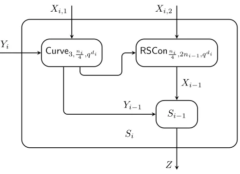
Definition 4.2.4 (inner sampler). For m ≥1, δ >0 and prime power q, picks =dlogme 3_{It is certainly not an exact equivalence since the parameters of extractors and samplers are slightly}

and let di = 2s−i for 0≤i≤s. Also let

ni =

 



16i 0≤i≤s−1,

max16s,20log_q(1/δ) i=s. DefineSi :Fnqidi ×Fdqi →Fmq for i∈[s] as follows:

• S0 :Fq×Fqd0 →Fmq projects (x, y) onto the first m coordinates of y.

• Si

def

= Si−1?RSConni/4,2ni−1,qdi

◦Curve_3,ni/4,qdi for i= 1, . . . , s.

Finally, let InnerSamp_m,δ,q def=Ss.

Figure 4.4 shows how Si is obtained from Si−1.

Si−1 RSConni

4,2ni−1,qdi

Curve_3,ni

4,qdi Yi

Xi,1 Xi,2

Xi−1

Z Yi−1

Si

Figure 4.4: The recursive construction of Si. Here Xi = (Xi,1, Xi,2) (resp. Xi−1) and Yi

(resp. Yi−1) are the two arguments of Si (resp. Si−1). And Z is the common output of Si

and Si−1.

Remark 10. We can check that all Si’s are well-defined. For S0 this is obvious. For i >1,

note that ni/4 is an integer. The function RSConni/4,2ni−1,qdi :F

ni/4

qdi ×Fqdi →F2_qndii−1 may be

viewed over _Fq:

RSCon_{ni/4,2ni−1,q}di :Fnqidi/4×F di

q →F

2ni−1di

q .

Given Si−1 :F 2ni−1di

q ×F2di

q →Fmq (notedi−1 = 2di), we have the function

Si−1?RSConni/4,2ni−1,qdi :F

nidi/4

q ×F

3di

q →F

The function Curve_3,ni/4,qdi :F3_qdini/4×Fqdi →F3_qdi may also be viewed over Fq:

Curve_3,ni/4,qdi :Fq3nidi/4×F di

q →F

3di

q .

Note thatSi = Si−1?RSConni/4,2ni−1,qdi

◦Curve_3,ni/4,qdi. So we have

Si :Fnqidi×F di

q →F m q

as claimed.

We then have the following theorem:

Theorem 4.2.2. For any , δ > 0, integer m ≥ 1 and sufficiently large prime power q ≥

mlog(1/δ)

O(1)

, let 0 =

2s and di, ni, Si be as in Definition 4.2.4. Then for each 0≤i ≤s,

the function Si :Fqnidi×Fdqi →Fmq is an (i, δi) manifold sampler of degreeti where i = 2i0,

δi =q−nidi/20, and ti =Qi_j=1(nj/4)2.

In particular, the function InnerSamp_m,δ,q : _Fn

q ×Fq → Fmq is an (, δ) curve sampler of

degree t where n ≤mO(1)_{+ 20 log}

q(1/δ) and t=O mO(logm)log

2

q(1/δ)

.

Proof. Induct oni. The claim is trivially true when i= 0. Now consider the case i >0 and assume the claim holds for all i0 < i.

By the induction hypothesis, Si−1 is an (i−1, δi−1) manifold sampler of degree ti−1. Then

by Corollary 4.2.2, Si−1?RSConni/4,2ni−1,qdi is an i−1+

0_{, q}(2ni−1−ni/4)di _{manifold sampler}

of degree (ni/4)·ti−1.

By Lemma 2.0.7,Curve_3,n

i/4,qdi is an

0_{, q}−nidi/16 _{curve sampler of degreen}

i/4. Then by

Lemma 4.2.3, the function

Si = Si−1?RSConni/4,2ni−1,qdi

◦Curve_3,ni/4,qdi

is an i−1+ 20, q(2ni−1−ni/4)di +q−nidi/16

manifold sampler of degree (ni/4)2·ti−1. It is then

just a routine to check the following facts:

i−1+ 20 = 2i0 =i,

q(2ni−1−ni/4)di_+q−nidi/16 _≤q−nidi/20 _=δ

i,

(ni/4)2·ti−1 =

i

Y

j=1

(nj/4)2 =ti.

Finally, note that InnerSamp_m,δ,q =Ss,=s and δ≥δs. So InnerSampm,δ,q :Fnq ×Fq →Fmq

is an (, δ) curve sampler of degree t where n = nsds ≤ mO(1)+ 20 logq(1/δ) and t = ts =