Development of a Multiple Degree of Freedom Knee Disarticulation Prosthesis with Active Leg Length Variation

http://dx.doi.org/10.4236/mme.2014.44020

Development of a Multiple Degree of

Freedom Knee Disarticulation Prosthesis

with Active Leg Length Variation

Berend Denkena, Martin Eckl, Dominik Brouwer

Leibniz Universität Hannover, Institute of Production Engineering and Machine Tools, An der Universität 2, Hanover, Germany

Email: [email protected], [email protected], [email protected]

Received 2 September 2014; revised 21 October 2014; accepted 6 November 2014

Copyright © 2014 by authors and Scientific Research Publishing Inc.

This work is licensed under the Creative Commons Attribution International License (CC BY). http://creativecommons.org/licenses/by/4.0/

Abstract

This paper presents a novel design for a knee disarticulation prosthesis. In this design, three hy-draulic cylinders form the supporting structure and provide the damping effect at the same time. That way the novel knee joint offers two fundamental advantages compared to the state of the art. First, the combination of a supporting structure and damping element reduces the weight of the prosthesis. Secondly, the use of several cylinders allows the actuation of further degrees of free-dom. Additional degrees of freedom can be used to vary the leg length within the gait cycle and hence to optimize the gait behavior.

Keywords

Biomechanics, Biomedicine, Prostheses, Knee-Disarticulation

1. Introduction

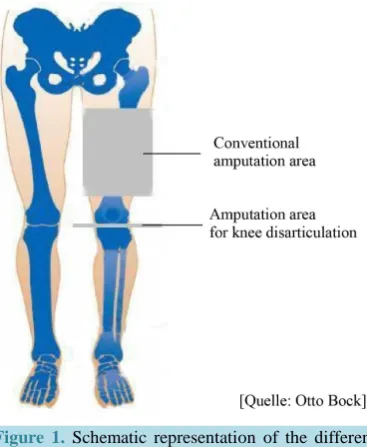
Exoprostheses are orthotics to balance functionality and cosmetic aspects of lost extremities. In the past 100 years the limb amputation indication changed from life saving measures due to injury to plastic, micro surgical intervention. The indication and the individual height of amputation influence the rehabilitation course. Hagberg

et al. show that the higher the level of amputation, the lower the degree of rehabilitation; hence a below knee amputation should be aspired [1]. Figure 1 shows the different amputation heights.

Figure 1. Schematic representation of the different

amputation levels.

keeps the ability to absorb the weight force as the ischial tuberosity is spared [3]. Furthermore, the knee disarti-culation does not affect the femur, and patella [4]. Thus, the remaining thigh muscles allow for coordinated stump movement [5]. In case of knee disarticulation, many different designs of the artificial knee joint can be applied. Stark gives a brief overview of such different designs [6]. In principle, any prosthesis for above knee amputees is suitable for knee disarticulation amputees as well. However, as the natural knee stump is still present, the artificial knee joint would be placed below the natural knee. These different anatomic situations need to be considered when selecting a knee joint design.

Current artificial knee joints are designed as single axis or polycentric joints. When single axis joints are used for knee disarticulation amputees, the distance between the anatomic and the artificial knee pivot point is long. This leads to an unnatural gait behavior and less stability within the walking cycle. O’Connor introduces a single axis joint where a special knee bracket reduces the distance between the anatomic knee and the pivot of the ar-tificial knee and provides a more naturally looking and operating prosthetic leg [7]. In contrast to single axis joints, polycentric knee joints are mainly used for knee disarticulation amputees. In this case, the pivot is varia-ble and outside of the actual knee joint mechanism. The design of such polycentric knee joints can be optimized to the requirements of knee disarticulation amputees. The University of Toledo has developed a method to op-timize a polycentric knee joint for knee disarticulation prostheses [8]. All current knee joints consist of a me-chanical supporting structure and an additional damping element.

In contrast, this paper presents a novel design for a polycentric knee joint for knee disarticulation prostheses, where hydraulic cylinders form the supporting structure and provide the damping effect at the same time (Figure 2).

The novel knee joint offers two fundamental advantages compared to the state of the art. First, the combina-tion of a supporting structure and damping element reduces the weight of the prosthesis. Secondly, the use of several cylinders allows the actuation of further degrees of freedom. Additional degrees of freedom can be used to vary the leg length within the gait cycle and hence to optimize the gait behavior. The patented design [9] was developed within the cooperative research project MultiPro, funded by the Federal Ministry for Research and Education (BMBF).

Figure 2.Design of the knee mechanism. (a) CAD model for different knee angles; (b) Knee mechanism within a gait cycle;

(c) Hydraulic system overview.

SimHydraulics (Mathworks). In Section 4 the hydraulic scheme is extended to enable active leg length variation within the gait cycle. The control scheme is simulated using Matlab/Simulink. That enables the simulation of a whole gait cycle with leg length variation. Finally, the development results of the research project are summa-rized in the conclusion.

2. Design of the Knee Mechanism

2.1. Description of the Novel Knee Mechanism

Figure 2(a) shows the CAD model of the artificial knee mechanism for different knee angles. The knee me-chanism consists generally of three linear hydraulic actuators. Two of the actuators are arranged symmetrically in the front of the prosthesis, while the third is arranged at the back of the prosthesis. Figure 2(b) illustrates the novel knee mechanism and a leg within the gait cycle (the kinematics of a gait cycle is shown in Figure 2). The left-top part of Figure 2 depicts how different angles are realized with the novel knee mechanism. To realize the knee of zero degrees, the front cylinders are at zero stroke and the back cylinder is at maximum stroke. To real-ize an angle, the forward cylinders are extended, the rearward cylinder is retracted. In this way, angles up to 120˚ can be realized. If the front cylinders and the rear cylinder are retracted, the length of the prosthesis is shortened, if all actuators are extended, the prosthesis is extended accordingly.

controlled leg length change, additional components have to be included. These components are described in Section 4. The change of the knee angle is driven by the external influences: hip movement, the patient weight force, and the ground reaction force. In the swing phase, the hip is moved forward and, thus, because of the iner-tia of the prosthesis, the prosthesis leg. In the stance phase the foot is fixed at the ground and the body is moved forward mainly by the hip movement. The ground reaction force and the movement of the hip generate a torque at the fork. So, in both phases of the gait, a counter direction movement of the rearward cylinder (cylinder 1) and the forward cylinders (cylinders 2 and 3) is generated. The fluid flows through the proportional valves 1 and 2 and the knee angle can be damped by adjusting the cross section of the valves to generate a sufficient torque in the stance phase and to control the correct knee angle in the swing phase. The damping value is set by propor-tional valves, depending on the current gait phase.

The invented knee mechanism is designed to sustain the mechanical stress, required by standard ISO10328

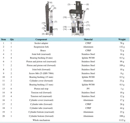
[10]. Most parts have been optimized using the Finite Element Method. If possible, lightweight materials have been used. The parts of the prosthesis, their materials and the corresponding mass are shown in Table 1. The knee mechanism has a weight of 1.115 kg while the whole prosthesis weighs 2.5 kg and is designed for patients with a maximum weight of 125 kg. A maximum knee angle of 136˚ is attainable.

Table 1. Overview of the components and its weights used in the knee joint.

Item Qty Component Material Weight

1 1 Socket adapter CFRP 78 g

2 1 Suspension fork Aluminum 132 g

3 1 Brace CFRP 72 g

4 2 Joint bolt (rearward) Stainless Steel 16 g

5 4 Bearing bushing (8 mm) Iglidur-W300 0.5 g

6 1 Piston and piston rod (rearward) Stainless Steel 99 g

7 2 Piston and piston rod (forward) Stainless Steel 109 g

8 2 Joint bolt (forward) Stainless Steel 10 g

9 2 Screw M6×25 (DIN 7984) Stainless Steel 8 g

10 2 Bearing bushing (15 mm) Iglidur-W300 0.5 g

11 2 Cylinder cover (forward) Aluminum 33 g

12 2 Bearing bushing (13 mm) Iglidur-W300 0.5 g

13 6 Piston end stop PV 1 g

14 8 Tension rod (forward) Stainless Steel 10 g

15 4 Tension rod (rearward) Stainless Steel 12 g

16 1 Cylinder cover (rearward) Aluminum 17 g

17 2 Cylinder tube (forward) CFRP 26 g

18 1 Cylinder tube (rearward) CFRP 44 g

19 1 Cylinder bottom (rearward) Aluminum 23 g

20 1 Cylinder bottom (forward) Aluminum 108 g

2.2. Controlling a Gait Cycle

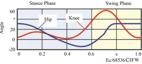
The required damping value depends on the gait phase. During the stance phase, the knee has to provide enough resistance to generate a sufficient torque to accommodate the weight force of the patient. While in the swing phase, the damping has to be low but adaptive to generate a natural looking swinging movement. Thus, control-ling a gait cycle requires the knowledge of the ground reaction forces in the stance phase, the current angle of the knee in the swing phase, and the desired movement of the knee. Any patient has his own pattern of move-ment, depending on the age, gender, body dimensions and, body proportions. Nevertheless, the general course of movement is nearly equal for any patient [11][12] and called gait cycle. The kinematics of the knee and the hip joint within the gait cycle are depicted in Figure 3.

The shown cycle begins with the stance phase. In this phase, the hip is at around thirty degrees, the knee is strait, and the foot touches the ground. While the foot is touching the ground, the hip is rotated back to approx. zero degrees and the knee is bended to approx. eighteen degrees. In this phase, the body is moved forward. In the swing phase of the illustrated leg (the other leg would conduct the stance phase), the hip is rotated to the starting position, while the knee has to be rotated to around sixty degrees to avoid collision of the toes with the ground.

The gait cycle begins with the stance phase while the foot is in contact with the ground. Within the swing phase, however, there is no contact between the foot and the ground. The lower part of Figure 4 shows the ho-rizontal

( )

( )

[12]-[18]. The upper part (right) shows a model of the location of the ground reaction force on the foot depend-ing on the gait cycle which was used for the simulations in this contribution. The point of application of the force vector depends on the gait phase. To be able to implement the ground reaction force in the simulation model, it is modeled as a superposition of the three vectors at the points of application (a a₁- ₃, Figure 4(b). The according vectors are weighted by the time dependent variables a t₁

( )

( )

( )

( )

( )

( )

( )

( )

( )

( )

B t =a t ⋅ B t + a t ⋅ B t + a t ⋅ B t =FH⋅ +x FV⋅ y

F F F F e e (1)

At the beginning of the stance phase the heel has the first contact with the ground: a₁ is 1, a₂ and a₃ are equal to zero. Within the stance phase, the point of application moves to the toes. In this way, at the end of the stance phase, a₃ is 1 and a₁ and a₂ are equal to zero (Figure 4(a)).

With the knowledge of the external influences within a gait cycle a control scheme is developed (Figure 5). The knee mechanism, presented in this paper, damps the leg movement hydraulically using proportional valves. As a control algorithm a fuzzy controller with 25 fuzzy rules is used to calculate the optimal damping value D_ϕ

depending on the gait phase and optimized by the optimization algorithm “active set” [19][20]. The input values of the fuzzy controller are the pressures inside the knee mechanism (P₁ and P₂), as well as the knee angle ϕ. It is necessary to convert the necessary damping value D_ϕ from the controller to the resulting damping values of the pistons. For this purpose, the direct kinematic is defined analytically according to the underlying geome-tric relations. The damping of the pistons is realized by adjusting the values of the hydraulic resistances (R₁ and

2

R ) of the valves 1 and 2.

The calculation of the knee angle ϕ from the measured piston positions is based on the inverse kinematic, which is, however, very complex to deduce analytically. Instead, discrete values of the inverse kinematic are identified using the CAD Software ProEngineer© and approximated by a fourth order Fourier transformation

Figure 3. Pattern of movement. (a) Curve of the knee angle;

Figure 4. Kinetic influence of the walking cycle. (a) Weight- ing of the points of action; (b) Locations of the points of

ac-tion; (c) Force curves within one gait cycle.

Figure 5. Control loop of the knee mechanism.

[21]. The calculation of the cross section of the proportional valves A_ν from the damping values of the pistons is derived in [22].

2 2 2

krit 3

4 2

π Re 16 Dr

A

R ν

ρ ν

α

= (2)

krit

Re is the critical Reynolds number

(

)

Figure 6. Test bed to investigate the knee mechanism.

Figure 7. Results of the verifications with the test rig.

the test rig show that a gait cycle can be performed with the developed control scheme. The piston movement occurs in counter direction as expected.

3. Compensation of Lateral Forces

3.1. Influence of Lateral Forces

The patient’s center of gravity is not directly above the knee joint. Thus, the displacement between the patient’s center of gravity and the knee d causes torque

( )

Figure 8. Force influence due to the patients weighty.

res weight 2 3

T =F d = −F a+F a (3)

weight 2 3

F =F +F (4)

However, since valves are passive elements, only damping forces (forces against the moving direction of the pistons) can be generated. Generating a force in moving direction, however, would require additional actuators. The necessary direction of the compensation force depends on the current load case, as shown in (5), and (6):

weight 1 2 2

d

F F

a

 _{− = −}

 

  (5)

weight 1 2 3

d

F F

a

 _{+ =}

 

  (6)

If the distance between the line of action of the weight force d is less than the distance between the pivot of the folk and the hydraulic cylinder a, then both compensation forces (F₂, and F₃) would act against the moving direction of the pistons and the whole torque T_res can be eliminated by controlling the valves. If d >a, however, the compensation force F₂ would have to act in the same direction as the piston movement. Since a force in that direction cannot be generated in a passive system, F₂ is set to 0 and a combination of mechanical and hydraulic absorption of lateral forces is required (7).

res weight 3 mech

T =F d=F a T+ (7)

mech

T is the torque, generated by the linear bearings. To estimate the actual lever arm d, the standard ISO 10328 [10] is used. The different test cases expect a lever arm d between 35 mm and 57 mm. The distance between the pivot of the fork and the cylinder a is 34 mm. Thus, in the worst test case (d = 57 mm), only 60% of the torque can be absorbed hydraulically and the linear bearing has to be designed to withstand 40% of the torque T_res.

3.2. Control Based Absorption of Lateral Forces

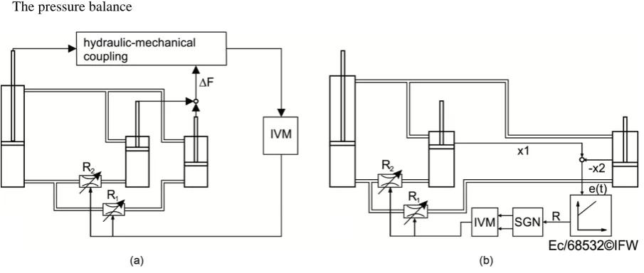
approach is an open loop control scheme (feed forward), wherein the forces are detected by force sensors and the necessary cross sections of the valves are calculated by a model of the hydraulic mechanical couplings (Figure 9(a)). The second control scheme is a closed loop control (feed back), wherein the difference of the piston position is detected and corrected by the valves (Figure 9(b)).

To realize the feed forward approach, the mathematical derivation of the mechanical and the hydraulic system in Figure 2 is presented while the mechanical system is loaded with the three forces F₁, F₂, and F₃.

The equations of motion of the cylinders are

1 1 12 2 1 1 1

m x = p A −p A−F (8)

2 2 22 2 1 1 2

m x = p A −p A−F (9)

2 3 32 2 1 1 3

m x = p A −p A −F (10)

where m₁ is the mass of the piston in cylinder 1 and m₂ is the mass of the pistons in cylinders 2 and 3. p₁,

12

p , p₂₂, p₃₂ are the pressures in the cylinder chambers (Figure 2(c)). A₁ and A₂ are the piston surfaces. The forces F₁, F₂, and F₃ are the loads acting on the piston rods Figure 9(b)). Due to the incompressibility of the fluid, stiffness effects can be neglected. The volume flow V₁ can be calculated as follows

1 1 1 2 1 3 1

V = −x A =x A +x A (11)

Therefore, the relation between position velocities is

1 2 3

x x x

− =  +  (12)

The damping effect is provided by the valves 1 and 2. The mathematical description of the valves is analogous to a hydraulic resistor. Macia and Thaler describe a hydraulic resistor R as the ratio of pressure difference ∆p and volume flow V [24].

p R

V

∆ =

 (13)

Using Equations (8)-(13) the dynamic behavior of the undamped hydraulic mechanical system can be de-scribed in the following way

(

)

(

)

1 2 1 2 2 1 2 2 3 2 1 2 3

x m +m =A R x +R x − F +F +F

   (14)

Based on that general system equation, the necessary relation between the resistors R₁ and R₂ of the valves to compensate the lateral forces is derived as follows.

The pressure balance is calculated by (9) and (10):

(

)

(

)

2 3 2 2 32 22 2 3

m x −x =A p −p +F −F (15)

The pressure balance

32 22 1 1 2 2

p −p =R V −R V (16)

As well as (13), and (15) lead to the dynamic behavior of the description of the dynamic coupling between the pistons.

(

)

(

)

3 2 2 1 2 2 3 2 3

2

1

x x A R x R x F F

m

− = − + −

    (17)

The pistons are constrained to equal speed:

2 3, 2 3 and 2 3

x =x x =x x =x (18)

The requirement (18) as well as (12) and (17) gives the relation between R₁ and R₂, which enables the compensation of lateral forces

3 2

2 1 2

2 1

2F F

R R

A x −

− =

 (19)

As an alternative to the feed forward approach, a feed back approach is presented, which determines the ne-cessary cross sections of the valves to compensate lateral forces from the difference of the piston positions of cylinders 2 and 3 by a PI control element. Therefore, the positions of the piston rods of the cylinders are meas-ured by displacement sensors and the difference of the two positions e t

( )

in-verse model of the valves (IVM).

For the investigation of both approaches a Matlab/Simulink model of the knee mechanism has been developed. The mechanical part is implemented by the SimMechanics toolbox, the hydraulic part is realized by the SimHy-draulics toolbox. In the simulation model the three pistons of the knee mechanism are loaded by different force steps. All force step occurs at the same time (after 0.07 s).

1

F is loaded with 1000 N, F₂ is loaded 800 N, and F₃ is loaded with 200 N. These test signals are chosen, because they show a high difference between the lateral forces F₂ and F₃. As a result, the three pistons move differently. The mechanical coupling of the pistons of cylinder 2 and 3 via the suspension fork as well as the mechanical support structure is not considered in these investigations.

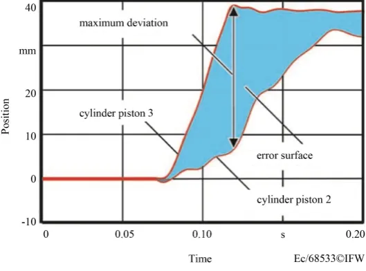
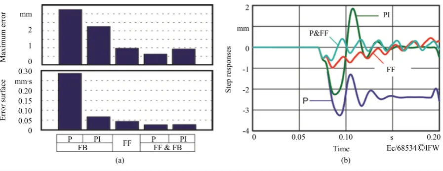
To be able to compare and evaluate the approaches to compensate lateral forces, an assessment scheme is de-veloped. The comparison values are the error surface and the maximum error (Figure 10). The goal is to mi-nimize both values. Figure 11 shows the results. Analyzed are the feed forward approach (FF), the feedback ap-proach (FB) with P and PI control element as well as combinations of both.

The column chart in Figure 11(a) a shows that the feed forward approach (FF) gives very accurate results.

Figure 11. Results of the compensation of lateral forces.

The feed back approach (FB) based on a P-control element is less accurate. The closed loop approach based on a PI-controller starts as accurately as the P-control element which leads to almost the same maximum error (Figure 11(b)). The I-control element, however, eliminates the steady state error which leads to an error surface less than the P-control element. The best results are achieved by superposition of the open loop control and the closed loop control.

The open loop control approach shows better results for two reasons: On the one hand, the closed loop control approach because a model of the process is implemented. On the other hand, that approach includes additional process information given by the force sensors. Thus, the control is able to act before an error occurs. The closed loop control approach, however, reacts after an error has occurred which leads to higher error values. The presented investigations are based on ideal assumptions. To evaluate the actual system behavior, it is necessary to consider delays of the valves, model inaccuracies, measurement inaccuracies and inaccuracies in the valves adjustments. These evaluations are presented in Section 3.3.

3.3. Investigation of Dynamic Influences and Interferences

The analyses in Section 3.2 assume ideal conditions. The actual valves, however, do not act immediately but delayed. This delay is approximated by a first order low pass characteristic. Figure 12 shows the maximum deviation in response to the time constant of the valves.

For short time constants the open loop control approach shows the best results. In this case, the process model is very accurate. For higher time constants the error increases rapidly, because the model of the process does not consider the valve behavior. However, for higher time constants, the closed loop approach shows better results due to the subsequent elimination of the additional error, caused by the dynamic behavior of the valves. The best results are achieved by superposition of both approaches. Current high response valves achieve a switching fre-quency of 125 Hz and a switching time of less than 3 ms, which is enough to generate good results as shows in

Figure 12.

In summary it has been shown that the hydraulic concept is able to absorb lateral forces, if the pistons of cy-linder 2, and cycy-linder 3 are loaded with forces with a positive sign (F₂>0, F₃>0). In combination with the mechanical bearings, all loads, based on [10] can be eliminated.

4. Active Leg Length Variation

4.1. Mathematical Description

The active variation of the leg length offers advantages for the patient. After an amputation the amputee is not able to lift his foot anymore. With the active variation of the leg length the patient is able to obtain more space between the moving foot and the ground. Thus, risks of collision and stumble can be reduced. The necessary energy to change the leg length is generated by the gait cycle. Thus, no external source of energy is required.

Figure 12. Influence of the valves dynamic.

posite direction changes the knee angle. Uniform movement of all three pistons, however, leads to the variation of the leg length. To enable uniform movement, the hydraulic scheme, depicted in Figure 2(c) needs to be ex-panded by an additional volume chamber to compensate the volume of the piston rods. The exex-panded hydraulic scheme is shown in Figure 13. In order to simplify the following calculations the valves 1 and 2 are summarized to the valve b. In that case the pressures in the chambers as well as the piston rods in the forward cylinders are equal.

This hydraulic scheme enables piston movements in opposite direction to change the knee angle as well as uniform motion to change the leg length. Superimposed motion of the angle and leg length is also possible. The directions of the movement of the pistons are adjusted by the two valves a and b by adjusting the cross sec-tion of the valves.

The shortening of the leg length happens in the stance phase and is driven by the weight of the patient. All three pistons move in negative direction

(

)

The valve b damps the opposite movement of the pistons of the backward and the forward cylinders and that way it damps the knee angle, while the valve a damps the uniform motion of the cylinders and controls the leg length variation. The mathematical description of the expanded hydraulic scheme is shown as follows:

a k k

V =A ⋅x (20)

2 2

b

V = A ⋅x (21)

1 2 b b p p R V − =

 (22)

1 k a a p p R V −

= _ (23)

where R_a and R_b are the hydraulic resistors of the valves a and b. The necessary value of R_b depends on the demanded motion of x₂ and is calculated by the Equations (21)-(22)

1 2 2 2 b p p R A x − =

 (24)

The necessary value of R_a is calculated by the Equation (20), and Equation (23) as follows:

1 2 a k k p p R A x − =

⋅ (25)

The Equations (24)-(25) enable the calculation of the values of the hydraulic resistances R_a, and R_b. These values lead to the demanded damping of the knee angle and the demanded leg length variation at the same time. The relation between hydraulic resistor and the adjustable cross section of the valve as well as the relation be-tween positions and the knee angle is depicted in Section 2.2.

4.2. Simulation of a Gait Cycle with Active Leg Length Variation

Figure 13. Extended hydraulic scheme.

inverse and direct kinematics are realized by Matlab/Simulink. This model allows simulating a whole gait cycle as depicted in Figure 14.

The actual ground reaction force and the influence of the torque from the hip are considered in this simulation model. The simulation shows that a gait cycle with active leg length variation can be realized with the presented knee mechanism. Figure 14 shows a gait cycle with leg length variation. The leg is shortened within the stance phase using the patient’s weight and it is lengthened within the swing phase using the force of the spring.

In the presented case, the leg length is varied by 10 mm. However, the curve of the leg length is just an exam-ple to show, that the actual leg length follows the desired leg length very well. The necessary curve of leg length variation is an anatomic challenge which has not been investigated yet.

Alternative to the presented hydraulic scheme, it is possible to realize leg length variation without an addi-tional energy store. In that case, within the stance phase, only the piston inside the backward cylinder is moving and that way the knee angle as well as the leg length is changing, while a volume chamber is filled. To extend the leg length within the swing phase, the kinetic energy of the leg is used.

4.3. Investigation of Dynamic Influences

The presented simulation assumes ideal conditions. Additionally, the influence of the low pass behavior of the valves is investigated using the assessment scheme, presented in Section 3.2. Here, the influence of the accuracy of the leg length variation of 10 mm is explored. The knee angle is not considered because the leg length variation is more sensitive than the knee angle damping.

Figure 15 shows the influence of the low pass behavior. The error of the leg length increases approximately linearly. A time constant of 0.02 seconds leads to an error of the leg length of 1 mm or 10% of the desired variation.

In general the influence of the valve behavior of the gait cycle as well as of the leg length variation is less than of the compensation of the lateral forces, because the lateral forces appear immediately.

5. Conclusions

Figure 14. Simulation of a gait cycle with leg length variation.

Figure 15. Influence of the valve dynamic of the leg length variation.

Since the only source of energy is the weight force, a leg length variation of 20 mm can be realized without ad-ditional actuators. By using the kinetic energy in the swing phase, it is also possible to realize active leg length variation without an additional spring energy store.

With the new prosthesis, a knee angle of 136˚ is attainable and it is designed to withstand a patient’s weight of 125 kg. The prosthesis complies with the standard ISO10328 and weighs only 2.5 kg.

Acknowledgements

The research studies, presented in this paper, have been part of the cooperation project MultiPro. The authors would like to thank the Federal Ministry for Research and Education (BMBF) for funding this project.

References

[1] Hagberg, E., Berlin, Ö.K. and Renström, P. (1992) Function after Through-Knee Compared with Below-Knee and Above-Knee Amputation. Prosthetics and Orthotics International, 16, 168-173.

[2] Behr, J., Friedly, J., Molton, I., Morgenrot, D., Jensen, M.P. and Smith, D.G. (2009) Pain and Pain-Related Interfe-rence in Adults with Lower-Limb Amputation: Comparison of Knee-Disarticulation, Transtibial and Transfemoral Surgical Sites. Journal of Rehabilitation & Development, 46, 963-972.http://dx.doi.org/10.1682/JRRD.2008.07.0085 [3] Greitemann, B. (2005) Kniegelenknahe Amputationen. In: Wirth, J.C. and Zichner, L., Eds., Orthopädie und Orth-

opädische Chirurgie, Georg Thieme Verlag, Stuttgart, 481-491.

[4] Baumgartner, R.F. (1979) Knee Disarticulation versus Above-Knee Amputation. Prosthetics and Orthotics Interna-tional, 3, 15-19.

[5] Mensch, G. (1983) Physiotherapy Following Through-Knee Amputation. Prosthetics and Orthotics International, 7, 79-87.

[6] Stark, G. (2004) Overview of Knee Disarticulation. American Academy of Orthotists & Prosthetists, 16, 130-137. [7] O’Connor, R.S. (1999) Prosthesis for Long Femur and Knee Disarticulation Amputation. Patent 5895430, USA. [8] Kramer, S., Srinivasan, S. and Swanson, V. (1998) Knee Joint Mechanism for Knee Disarticulation Prosthesis. Patent

5746774, USA.

Prosthe-sis for Human Leg, Has Hydraulic Assemblies Causing Motion of Artificial Replacement Member of Leg Sections around Rotary Axis by Movement in Opponent Arrangement. Patent DE102009056074A1, Germany.

[10] ISO10328:2006 (2006) Prosthetics-Structural Testing of Lower-Limb Prostheses-Requirements and Test Methods. [11] Perry, J. and Burnfield, J. (1992) Gait Analysis: Normal and Pathological Function. Slack, New York.

[12] Whittle, M.W. (1996) Gait Analysis: An Introduction. Butterworth-Heinemann Ltd., Oxford.

[13] Al-Hamadi, A., Andres, S., Berndt, D., Calow, R., Lehmann, C., Michaelis, B., Schünemann, S. and Urbansky, U. (2004) 3D-Bewegungsanalyse in der “Neuro-Medizintechnik”. Ph.D. Dissertation, Otto-von-Guericke-Universität Magdeburg, Magdeburg.

[14] Götze, C., Sippel, C., Rosenbaum, D., Heckenberg, L. and Steinbeck, J. (2003) Objective Measures of Gait Following Revision Hip Arthroplasty. First Medium-Term Results 2.6 Years after Surgery. Zeitschrift für Orthopädie und ihre Grenzgebiete, 141, 201-208.

[15] Seichert, N., Erhart, P. and Senn, E. (1997) Die Etablierung der instrumentierten Ganganalyse (IGA) als Verfahren zur unmittelbaren klinikrelevanten Gangbeurteilung.Darstellung der propulsiven und bremsenden Muskelaktivitäten beim Gehen. Physikalische Medizin, Rehabilitationsmedizin, 7, 1-11.

http://dx.doi.org/10.1055/s-2008-1061850

[16] Kramers-de Quervain, I.A., Stüssi, E. and Stacoff, A. (2008) Ganganalyse beim Gehen und Laufen. Schweizerische Zeitschrift für Sportmedizin und Sporttraumatologie, 56, 35-42.

[17] Leuchte, S. and Luchs, A. (2006) How Symmetrical or Asymmetrical Is the Physiological Gait in Respect of Age?

Journal of Physical and Rehabilitation Medicine, 16, 96-102.

[18] Hölscher, C. (2009) Auswirkungen Von Hohen Tibialen Umstellungs-Osteotomien auf den Gang und die Kniegelenks- Belastung. Ph.D. Dissertation, Medizinische Fakultät der Westfälischen Wilhelms-Universität Münster, Münster. [19] Fletcher, R. (1987) Practical Methods of Optimization. John Wiley & Sons Limited, West Sussex.

[20] Gill, P.E., Murray, W. and Wright, M. (1982) Practical Optimization. Emerald Group Publishing Limited, London. [21] Sneddon, I.N. (1995) Fourier Transforms. Dover Publications, Inc., New York.

[22] Clarke, J.A. (1985) Energy Simulation in Building Design. Butterwort-Heinemann, Oxford.

[23] Crane Co., NY. (1982) Flow of Fluids through Valves, Fittings and Pipes. Metric Edition-SI Units, Technical Paper No. 410M, Crane Co., New York.