Voluntarily Relinquishing Private Property Rights: The Existence of Risk Pooling Equilibria When Facing Environmental Uncertainty

http://dx.doi.org/10.4236/tel.2015.52027

How to cite this paper: Raymond, F.E. and Raymond, B.W. (2015) Voluntarily Relinquishing Private Property Rights: The Ex-istence of Risk-Pooling Equilibria When Facing Environmental Uncertainty. Theoretical Economics Letters, 5, 225-237. http://dx.doi.org/10.4236/tel.2015.52027

Voluntarily Relinquishing Private Property

Rights: The Existence of Risk-Pooling

Equilibria When Facing

Environmental Uncertainty

Francis E. Raymond

1

, Benjamin W. Raymond

2

1_{Department of Economics and Finance, Rubel School of Business, Bellarmine University, Louisville, KY, USA} 2_{Department of Economics, Krannert School of Management, Purdue University, West Lafayette, IN, USA} Email: [email protected], [email protected]

Received 15 February 2015; accepted 25 March 2015; published 31 March 2015

Copyright © 2015 by authors and Scientific Research Publishing Inc.

This work is licensed under the Creative Commons Attribution International License (CC BY). http://creativecommons.org/licenses/by/4.0/

Abstract

As weather patterns across the globe change in response to global warming, we should expect more strain on existing institutions. This paper demonstrates how weather risk induces farmers into a risk-pooling equilibrium whereby private property rights are voluntarily relinquished. We find that as the spacial variability of rainfall increases, rising investment and increased subplot dispersion are complementary hedges against weather risk. With subplot dispersion, the cost of preserving private property rights rises, incentivizing farmers to develop a system of common property rights. In contrast, investment and subplot dispersion become substitute hedges as weather risk diminishes. We provide a dynamic theoretical model which complements previous empirical work on the impact of weather risk on property rights.

Keywords

Global Warming, Common Property Rights, Risk-Pooling, Spacial Variability, Dynamic Programming

1. Introduction

226

Sethi and Somanathan [3] describe the impact of various property rights regimes on social cohesion and re-source exploitation. Moreover, private property rights that are enforced by law are considered to be the founda-tion for both entrepreneurship and market efficiency [4] [5].

In a strategic model of cooperation, Tornell [6] studies the connection between shifting property rights re-gimes and economic growth. Under special assumptions the author generates equilibria with perpetual common property rights. This, Tornell argues, may help to explain the sluggish development observed in lesser developed countries. By holding private property as collateral, individuals are able to secure loans and insurance, enabling them to smooth consumption streams over time. Collateral also stimulates entrepreneurship by providing the necessary financial means and reducing the short run risk associated with undertaking new ventures. Van Long and Sorger [7] prove that when political institutions are weak, rising transactions costs reduce the incentive to covert common property into private capital, thus reducing productivity and growth. However, stressful political, economic or environmental situations can lead individuals to willingly forgo private property rights. Of particu-lar interest is the influence of external factors on the formation of alternative types of property rights regimes. In particular, when might individuals’ incentives favor dissolving private property rights in favor of common prop-erty rights?

According to Coase [5] the assignment of property rights allows bargaining, and thus contributes to allocative efficiency. Acheson [8], Li [9], and De Zeeuw [10] each describe various types of communication and bargain-ing that facilitate the evolution of inter and intra-community agreements concernbargain-ing the optimal management of common property resources. Cultural norms can significantly affect the way in which individuals and groups respond to uncertainty. In a study of traditional property rights in the arid regions of Africa, Goodhue and McCarthy [11] find that even in the midst of violent conflicts and government sponsored privatization, tradi-tional views concerning the value of mobility, as well as the right of exclusion, remain important. These norms also influence perceived social and economic benefits of private property rights, either enabling or stunting a transition to a system of shared property rights.

In Honduras, Tucker [12] shows that a socially optimal allocation of clay for pottery production occurs when the benefit of pooling is substantial and obvious to the community. Under these circumstances communities will develop institutions supporting communal access to a normally private resource. In a two-stage game, Chiang and Li [13] demonstrate that within a chaotic environment where production is uncertain, any transition from private to collective property rights depends in part on players’ willingness to enforce private property rights.

Using panel data from rural India, Rozenzweig and Binswanger [14] demonstrate the impact of changes in weather patterns on investment returns and the stability of consumption. By developing and testing static first order conditions for utility maximization they demonstrate that the benefits of weather related insurance would be significant if it were universally available and affordable. However, in the absence of weather related insur-ance, farmers must rely upon other risk reducing measures.

McCloskey [15] demonstrates that environmental factors help determine optimal property rights regimes. In particular, she focuses on the impact of intertemporal and spacial variation in rainfall on individuals’ willingness to maintain private property rights. Intertemporal variability describes changes in the amount of rainfall over time. Generally speaking, prolonged droughts affect intertemporal variability. Spacial variability differs from intertemporal variability in that even if an area receives an average amount of rainfall, certain sub-regions might experience drought conditions while others in close proximity with it experience more plentiful rainfall. In em-pirical studies involving Sub-Saharan Africa Nugent and Sanchez [16] [17] show how spacial variability can lead tribal farmers to forgo private property rights in favor of a hybrid regime involving common property rights. Nugent and Sanchez assume that farmers’ utility is based upon average crop yield and rainfall variability. When environmental risks such as spacial variability of rainfall increases (variation according to location), there is an incentive to scatter the plots of land under their control. As a result, tribes become increasingly nomadic. This suggests that there is a threshold where the benefits associated with mobility outweigh those of land ownership. Moreover, once this threshold is reached, individual tribes seem to simultaneously relinquish their squatters’ rights in favor of a regime of common property rights where all tribes are allowed access to property formerly controlled by a single tribe.

227

depends on technologies of production and enforcement and on the values of inputs and outputs. In some cir-cumstances the costs so obviously exceed the benefits that it is not in the social interest to create property rights over a particular class of resources (p. 562).”

Crépin and Lindahl [19] use a somewhat similar dynamic approach to illustrate examples of either coopera-tive or non-cooperacoopera-tive behavior when managing grasslands. In contrast, our model completely characterizes the dynamics of a pooling equilibrium when weather risk is increasing, and when it is decreasing. The analysis herein provides a theoretical approach to analyzing the influence of weather risk in determining property rights. If weather risk is increasing, one would expect utility to rise as farmers subdivide land endowments into dis-persed subplots as long as the net benefits from dispersing land into subplots exceeds the net benefits from maintaining private property rights. In order to facilitate subplot dispersion, the individual farmer must enter into land-swap negotiations with his neighbors. This is the first step in relaxing control over the initial endowment of land. In addition, as the number of subplots grows, the cost of maintaining private property rights rises. The in-dividual farmer is forced to relinquish more control until it is no longer in his interest (utility maximizing) to at-tempt to maintain private property rights. At this point, the region enters into a common property rights regime. In contrast, when weather risk is declining, the benefits accruing to the enforcement of private property rights exceed the benefits of dispersing land into subplots, so private property rights are sought and enforced.

The literature concerning spacial variability of rainfall has been predominantly descriptive, static and empiri-cal. The models define farmers’ utility in terms of consumption and risk avoidance without explicitly incorpo-rating production and costs. Despite the fact that the models are static, there appears to be a desire to extrapolate the results over time. This comes from the fact that property rights do not evolve instantaneously. Weather pat-terns tend to change gradually, and people’s responses to these changes are measured.

What follows is an intertemporal mathematical model illustrating conditions that motivate groups to forego private property rights in favor of common property rights. In short, the model investigates the impact on prop-erty rights regimes of the spacial variability of rainfall over time while considering production and costs. The model provides a theoretical framework to complement previous empirical analyses, particularly those of Nu-gent and Sanchez [16] [17].

From a policy perspective, fully understanding the circumstances surrounding the evolution of property rights regimes is important when formulating appropriate policies aimed at the development of nations where weather conditions are less predictable. This model helps to explain why different regimes may exist, thus guiding policy makers entrusted with fostering economic development in arid and semi-arid nations to create appropriate laws, and to effectively allocate subsidies. For example, laws and subsidies incentivizing the accumulation of private property may be ineffective and wasteful, especially if these same laws undermine the potential for the formula-tion and management of common property.

The paper contains four primary sections. Following the introduction, section two provides the intuition and de-tails of the model. Section three explores the dynamics of property rights regimes and section four concludes the paper.

2. Model

Risk averse farmers coexist in an region where they are subject to spacial variations in rainfall. Increases in the spacial variability of rainfall increase the risk to farming and decrease land values. As a result, the ability to se-cure insurance or credit decreases, even from informal sources. Weather risk is hedged by crop diversification, mixing farming with animal husbandry, increasing hoarding and saving, and risk pooling via plot scattering or nomadism. Farmers are motivated to disperse their plots over a wider region. Attempting to maintain private property rights while dispersing plots results in higher transportation costs, transactions costs and storage costs. There are also higher costs associated with monitoring and enforcement of private property rights. Further di-versification increases these costs, arguably at an increasing rate. Thus, one would expect farmers to gradually begin to support a system favoring open access.

We assume that individual farmers are each endowed with property rights to equally sized single plots

( )

Hi

228

or grazing. In fact, it is the pursuit of farming or grazing opportunities in the face of increasing weather risk that motivates farmers to relax or relinquish private property rights. By relinquishing private property rights, those benefits that are specifically tied to property ownership are forgone. Therefore, as spacial variability in rainfall increases, there is a trade-off between the benefits (profits) ones accrues from farming and those benefits spe-cific to land ownership.

We assume that within a given region, there is a representative agent or farmer seeking to maximize utility,

( )

,

u

π

b , over time. Profit from farming or grazing is

π

. The parameter b summarizes the net benefits of maintaining private property rights. Assume that u

( )

π

,b is increasing and concave in both arguments. This includes benefits such as the ability to use as collateral, while also considering costs to maintain these rights. Again, the benefits and costs associated with preserving property rights are considered separately from those specifically associated with farming. To fully comprehend the parameter b, simply subtract the profits that would typically accrue to a tenant-farmer from the profits and other net benefits one would receive as an owner- farmer. As the number of subplots increases, monitoring becomes more difficult and incidences of squatting, crop seizures and even vandalism are likely to increase. It is assumed that these costs would affect the tenant farmer and the owner-farmer similarly. Thus, the parameter b is assumed to depend indirectly on the number of subplots, m.

2.1. Considering Weather Risk

The farmer has the option to hold his land endowment (H) in the form of a single plot. However, he can also choose to reduce his exposure to weather related risk by subdividing his land endowment into m subplots

(

H ii, =1,,m

)

which he can then exchange for comparable subplots throughout the region. The farmer’s total property can then be expressed as H=

∑

_im₌₁H_i. Define σ2 to represent the spacial variability of rainfall within the region. As the spacial variability of rainfall falls, there is less incentive to scatter plots, because doing so is costly. However, as σ2 rises, farmers have a greater incentive to engage in negotiations with neighbors in an effort to exchange small subplots of land among one another.

Assume that spacial variability has constant variance within a region. Thus, σ2 does not vary across sub-plots. However, the correlation in rainfall

( )

r_jk between subplots Hj and Hk, will be higher the closer the

subplots are to each other, and lower the further away they are. With this in mind, as in Nugent and Sanchez (1999, p. 270), define

(

)

(

)

2 2

1 1

R m r

m

σ

σ = + − (1)

as the average variance of rainfall across all subplots held by the representative farmer, where 0< <r 1 de-notes the mean of all pairwise correlation coefficients.1 In fact,

σ

_R2 quantifies the risk faced by the representa-tive farmer. As weather risk

( )

2

R

σ increases in response to increases in the spacial variability of rainfall

( )

σ2 _,

farmers increasingly look to subplot dispersion to reduce this risk. Assuming differentiability as needed, it fol- lows that

(

)

(

)

2

2

1

1 1 0

R _{m r}

m

σ σ

∂

= + − >

∂ (2a) And

( )

2 2

2 2

1 0,

R r

m m

σ σ

∂ ₋

= <

∂ ∂ (2b)

so the benefits one earns from increasing plot dispersion in the face of growing spacial (regional) variability de-creases with m. Moreover,

(

)

2

2

1 0

R r

m m

σ

σ −

∂

= <

∂ (3a)

1_{Equation (1) provides a foundation for McCloskey (1989), ands Nugent and Sanchez [16] [17]. Thus, it is desirable to also use it for this}

theoretical model. Note, when 2 2

229

and

( )

(

)

2 2

2 3

2 1

0.

R r

m m

σ σ

∂ − −

= >

∂ (3b)

So, even when spacial (regional) variability is constant, increasing subplots has a diminishing impact on risk. Also note that the average variation in rainfall, r, rises as the number of subplots, m, rises because as the sub-plots become more dispersed, there is greater variation in the weather between sub-plots, and average variation rises.

Assume a perfectly competitive market for an agricultural capital-consumption good, x, and an exogenously determined price, p. Again, m is the extent to which land is divided into subplots (and exchanged). One manages weather risk,

σ

2_R, by choosing m. Production, f x

(

,σ_R2

( )

m

)

, is increasing and concave with respect to the cap-ital consumption good, x, and decreasing and convex with respect to risk,

σ

_R2

( )

m .2 Define x to be invest-ment, or the change in the input x (e.g. seed), to be employed in crop production in the next period once quan-tity supplied

( )

q is determined and depreciation

( )

ζ

x is taken into account.3 As a result, crop production follows the growth rule,

( )

(

2

)

, R .

x= f xσ m − −q ζx4 (4) In this model, ex ante, the farmer chooses a fixed percentage of the available crop

( )

ζ

x for personal con-sumption. The farmer endogenously determines the amount of the crop he wishes to supply (q). Total costs are defined by C m

( )

= +c₀ c m

( )

where c m

( )

represents the transportation, transactions, and private property enforcement costs associated with plot scattering and c₀ represents fixed costs (tools etc.) not directly related to plot scattering. Assume the marginal cost associated with plot dispersion increases at an increasing rate, so

2

2

0 and 0.

m mm

c c

c c

m m

∂ ∂

≡ > ≡ >

∂ ∂

5

In conjunction with 2

lim _R

m→∞σ =σr, this condition on costs ensures that there exists some

0 0

m ≥ such that for 0

m>m , the net benefit associated with increasing the number of subplots while maintaining private prop-erty rights is zero. Thus, there are limited benefits to maintaining propprop-erty rights as subplots become more dis-persed. Eventually, the farmer will reach a number of subplots, * 0

m ≤m , where private property rights are vo-luntarily surrendered in favor of a common property rights regime.

The farmer’s profit function is

π

= pq c− −₀ c m

( )

where price, p>0, is exogenously determined. Addi-tional net benefits accrue to the farmer who maintains property rights. Define b=b

(

σ_R2

( )

m

)

. Thus, the net benefit associated with land ownership depends on the average variability of rainfall which can be influenced by dispersing one’s land into subplots. It follows that

2

2 _R 0,

R

b b_σ

σ

∂ _{≡ <} ∂

2

2 0.

R m

R

b b

b

m m

σ σ

∂

∂ _{≡ =} ∂ _>

∂ ∂ ∂

Again, this assumes that there are limits to which risk can be offset and benefits can accrue as crops are dis-persed.

In the presence of weather risk, an increase in the number of subplots (m) decreases the variability in crop yields (Equation (2b)). This should increase the total value of

1 ,

m i i

H=

∑

₌ H including the net benefits of

2

Production,

(

2

)

, R

f xσ , has the properties f >0,fx>0,fxx<0, 2 0, 0,22

R RR

f_σ < f_{σ σ} < and 2 2>0

Rx xR

f_σ =f_σ .

3_{Corn is an example of an agricultural capital consumption good, for it can be consumed, or it can be invested (saved as seed for the next set} of crops).

4_{This is an intentionally different interpretation of Solow’s law of motion (1956). In the law of motion depicted here, the farmer manages the}

quantity to be sold (q) in lieu of consumption. Consumption is a constant percentage of the total capital-consumption good available, ζx. There is no depreciation.

5_{As long as the notation is clear, we opt to express derivatives like} 2 R b

δ ∂σ , using the notation 2

R

b_σ . One noteworthy exception is that

derivatives of 2 R

σ will be expressed as 2

R m

σ δ

∂ , etc. Also, we adopt the following notation denoting the time derivative, m =δ δm t,

230

maintaining private property rights. However, if utility rises by increasing the number of subplots, the region moves closer to a system of common property rights when the number of plots reaches m*. Therefore, an in-crease in the spacial variability of rainfall

( )

σ2 increases weather risk, motivating farmers to reduce this risk by increasing the number of dispersed subplots, and eventually surrendering private property rights.

2.2. Intertemporal Utility Maximization

Because voluntarily relinquishing property rights is necessarily an evolving process, we investigate the problem from an intertemporal perspective. This is consistent with the fact that weather risk changes gradually, so sub-plot dispersion occurs slowly, with the number of subsub-plots increasing gradually as the weather becomes less predictable. As weather conditions become riskier, the number of subplots grows and subplots become more dispersed; eventually farmers may decide that the costs associated with maintaining property rights exceed the benefits. This progression is not addressed by the existing empirical work.

The representative farmer chooses the quantity to be sent to market and the number of subplots in a manner consistent with intertemporal utility maximization. Thus, assuming β is the discount rate and suppressing the time argument, t, the farmer’s intertemporal utility maximization problem is:

(

)

(

( )

)

(

2

)

0 ,

max e t , , d

R

q m u q m b m t

β _{π σ}

∞ −

∫

Subject to

( )

(

2

)

, _R ,

x= f xσ m − −q ζx

with the additional condition that,

(

)

(

)

2 2

1 1 .

R m r

m

σ

σ = + −

Assume for simplicity that utility is derived directly from the profits and the net benefit of property ownership. The farmer’s problem then becomes:

( )

(

( )

)

(

2

)

0 0

,

max e t R d

q m pq c c m b m t

β _σ

∞ − _{− − +}

∫

(P)

Subject to

( )

(

_, 2

)

R

x= f xσ m − −q ζx (5)

with the additional condition,

(

)

(

)

2 2

1 1 .

R m r

m

σ

σ = + − (6)

The control variables of this optimal control problem are q and m. The state variable is x.

3. The Dynamics of Property Rights Regimes

In order to generate the first order conditions for a maximum, formulate the current value Hamiltonian:

( )

(

2

( )

)

(

(

2

( )

)

)

0 R , R .

H = pq− −c c m +b σ m +λ f xσ m − −q ζx 6 (7)

The partial derivatives yield two first order conditions, Equations (8) and (9).

0

set q

H

H p

q λ

∂

≡ = − =

∂

so, λ=p.7 (8) Also,

6_{The reader can verify that the second order derivatives have the appropriate sign for a maximum.} 7_{When convenient, we adopt the convention,}

q

231

2 2

2 2

0,

R R

set

R R

m m

H

H c b f

m σ m σ m

σ _λ σ

∂  ∂ 

∂

≡ = − + _{ }+ _{ }=

∂ _ ∂ _{ } ∂ _

so,

(

2 2

)

2

.

R R

R

m

b f c

m σ σ

σ _λ

∂

+ =

∂ (9)

According to Equation (9), optimal plot diversification occurs when the marginal benefit of diversification, in terms of the impact of rainfall variation has on both benefits of ownership and production, exactly offsets the marginal cost of plot diversification.

The current value adjoint or costate equation is:

(

fx

)

fx.

λ βλ λ

= − −

ζ

⇒ = + −

λ β ζ

 (10)

Combining (8) with (10), when

λ

= =p 0, it follows that f_x− =ζ β. That is, the marginal increase in cap-ital equals the discount rate, or the rate of impatience. Note that farmers in this scenario most likely face a com-petitive market, so price changes are exogenous. Thus, in the absence of significant external shocks, price will remain relatively constant.

Recall that supply follows from Equation (4),

( )

(

_, 2

)

_.

R

q= f xσ m −ζx−x

The steady-state exists when investment is constant

(

x=0

)

. Thus, in the steady-state,

( )

(

2

)

, _R .

q= f xσ m −ζx

Differentiate this expression for x, employing Equation (10) when

λ

= =p 0. We see that in the steady state,

.

x x

q = f − =ζ β (11) Thus, in the steady-state

(

x=0

)

, when price is constant

(

p =0

)

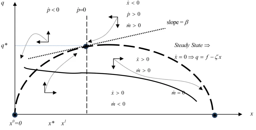
the optimal level of capital, *

[image:7.595.90.540.475.704.2]

x , satisfies the condition that the marginal propensity to sell another unit equals the opportunity cost of foregone capital (as indicated by discount rate). In Figure 1, we illustrate this version of the familiar rule governing the optimal cap-ital stock, x*.

Figure 1.Steady-state optimum when 2

0

232

3.1. Optimal Subplot Diversification

The following illustrates the conditions that determine the optimal number of subplots given rainfall variability, and the marginal benefits and marginal cost of diversification.

Proposition 1: The optimal number of diversified subplots is positively related to the spacial variability of rainfall, and varies inversely with respect to the marginal cost of subplot diversification.

Proof: To determine the optimal number of subdivided and dispersed plots, substitute for ∂

σ

_R2 ∂m in the second first order condition (9) to obtain,

(

)

₍

₎

2 2 2 2 1 .

R R m

r

b pf c

m σ σ

σ −

+ =

Solve for m to obtain the optimal number of subplots,

(

)

(

2 2

)

1 2 2 1 0. R R m

r b pf

m c σ σ σ  _{− +}   

=_{ } >

 

 

(12)

The result then follows directly from Equation (12). ■

3.2. Optimal Investment and Production

We now wish to examine the dynamics of the farmer’s problem (P) in more detail. Differentiating the mean va-riability of rainfall (or weather risk) given by Equation (1) with respect to time, one sees that the average varia-bility of rainfall witnessed by the farmer changes over time according to the rule,

(

)

(

)

(

(

)

)

2

2 2

1 1

ˆ 1 1 1 ,

R _{m r m r}

t m m

σ _{σ σ}

∂

= − + + −

∂  (13)

where

σ

2 = ∂

σ

2 ∂t.

Next, assume that r is constant over time, so r=0. Then (12) combined with the time derivative of weather risk (13) we see that,

(

2 2

)

(

2 2 2 2

)

2 2

2 2 2 2 2 2

2 _{R R R R R R R R}.

R R R R R

mm _x

m b pf c b pf pf x pf

m t m m

m σ σ σ σ σ σ σ σ

σ σ σ σ σ

∂  ∂ ∂ ∂ ∂ + − = − + − −   ∂ ∂ ∂ ∂ ∂  

   (14a)

After solving for x, we obtain optimal investment,

(

2 2

)

(

2 2 2 2

)

2

2

2 2 2 2 2

2

2 .

R R R R R R R

R

R R R R

mm

R x

c b pf m b pf pf

m t m

m x

pf m

σ σ σ σ σ σ σ

σ

σ σ σ σ

σ  ∂  ∂ ∂ ∂ − + − + −  _∂  _{∂ ∂ ∂}   = ∂ ∂   

Using Equation (13), substitute for

2

R

t

σ

∂

∂ above. Then, (14b) reveals another condition for optimal investment,

(

2 2

)

(

2 2 2 2

_{) (}

₎

2 2 2 2 2

2 2

2

2

2 2 2

2 2 2

2

ˆ .

R R R R R R

R R R R R

R R

R

R R

mm

R

R _{x x}

x

c b pf b pf m

b pf

m

m f p

x

pf f

pf m

σ σ σ σ σ σ

σ σ σ σ σ

σ σ σ σ σ σ σ σ  _{∂ ∂ }   − + −_{ } +  + ∂ ∂  _{ }    = − − ∂ ∂  

 (14b)

This solution to the Hamiltonian system yields the optimal condition for investment. Equations (14a) and (14b) define the optimal conditions consistent with intertemporal utility maximization.

233

( )

(

)

(

)

(

)

(

)

2 2 2 2 2 2

2

2 2 2 2 2

2 2

2

2 2 2

2 2 2 2 2 , ˆ + .

R R R R R R

R

R R R R R

R R R R mm R R x R x x

b pf c b pf m

m m

q f x m x

pf m

b pf f p

pf f

σ σ σ σ σ σ

σ

σ σ σ σ σ

σ σ σ σ σ ζ σ σ σ _{∂ ∂ }   + − +_{ } +  ∂ ∂  _{ }    = − + ∂ ∂ + +   (15)

Proposition 2: As a hedge against weather risk, (a) optimal investment is positively related to changes in the spacial variability of rainfall. Consequently, optimal quantity supplied is negatively related to variations in the spacial variability of rainfall. (b) In contrast, optimal investment varies negatively with subplot diversification, while optimal quantity supplied varies positively with subplot diversification.

Proof: (a) By our initial assumptions,

( ) ( )

( )

2 2 2 2

2

2

0

R R R R

R

R

x

b pf

pf

σ σ σ σ

σ σ+ − +   +  

  _<

,

And

(

)

( )

( )

2 ₂ 2 2 2 2

2 2

2 2 2

2

2 0.

R _R R R R R

R

R R

mm

R x

b pf c b pf

m m

pf m

σ

σ σ σ σ σ

σ σ σ σ − −   ∂  ₊ _{− +} ∂ ₊     _∂ ∂   _{ } > ∂ ∂

Then, result (a) follows directly from Equation (14b) and result (b) follows directly from the expression above and (15). ■

Therefore, if the farmer chooses to maintain the current number of plots, when spacial variability increases, the farmer will choose to reduce the quantity supplied and increase investment, x. In other words, if the num-ber of plots is fixed, the farmer devotes a greater share of his crop toward seed as a hedge against greater uncer-tainty.

3.3. Subplot Dispersion in the Steady-State When Average Variability of Rainfall Is Rising

By definition, subplot dispersion is constant if m =0. We gather information about subplot dispersion by first investigating the steady-state when m =0. Recall that the steady-state level of capital is defined by x=0. In the steady-state, Equation (4) becomes,

( )

(

2

)

, _R 0,

x= f xσ m − −q ζx=

or, q= f x

(

,σ_R2

( )

m

)

−ζx. (16)

Thus, Equation (16) defines the steady-state condition, x=0. When m =0, Equation (15) becomes

( )

(

)

(

2 2 2 2

)

2

2 2

2 2 2

ˆ

, R R R R R .

R R

R R

x x

b pf f

q f x m x p

pf f

σ σ σ σ σ

σ σ

σ σ

σ

ζ

+

= − +  + (17)

Equation (17) describes the path m =0 in terms of x and q. Again, by identifying when subplot dispersion is constant

(

m =0

)

, we can determine whether the farmer is increasing

(

m >0

)

or reducing

(

m <0

)

the num-ber of subplots in the steady-state. One can see from Equation (15) that when m <0, the value of q is less when

0

m = . Similarly, when m >0, the value of q is greater than it is when

0

dis-234

persion whereas below the curve, there is a tendency to decrease dispersion.8

Next, we study the effect on subplot dispersion when the spacial variability of rainfall is increasing

(

σ2>0

)

and then when it is decreasing

(

σ2<0

)

. First, assume that the spacial variability of rainfall is increasing.

Also note that,

(

( )

)

( )

2 2 2 2

2

2 2 0.

R R R R

R

R

x

b pf

pf

σ σ σ σ

σ

σ σ

−

+

+

<



(18)

Thus, Equation (17) demonstrates that the path of m =0 lies below the steady-state x=0 when price is constant

(

p= =pˆ 0

)

. Because 2 2 0

R x R

f_σ f_σ < , the same is true when price is rising. Moreover, in this scenario, it is likely that increased weather risk reduces market supply, causing price to rise. As a result, it is far more likely that p ≥0, and hence pˆ≥0, although we also show the case when price is falling

(

p <0

)

.

Recall that by Equation (11), when p =0, the optimal level of capital, x*, is defined by q_x =β in the steady-state. Naturally, we are most interested in the case where the average variability of rainfall is rising

(

2

)

0

σ > . Figure 1 illustrates the steady states when this weather risk is increasing. It follows that as σ2 rises, the path of m =0 shifts down, further away from the steady-state. With respect to Figure 1, the steady-state condition is defined by x=0. Since the objective function is linear in q, it is a “bang-bang” control variable. As such, the farmer will choose to either sell nothing, or sell q*.

Since x= f x

(

,σ_R2

( )

m

)

− −q ζx, at any given value for x, a reduction in q implies x rises. Thus, x>0

below the steady-state condition x=0. Similarly, x<0 is above the condition x=0. In addition, according to Equation (15a), when price falls below p*, quantity supplied falls to zero. Therefore, the optimal amount of capital, x* associated with q*, is a utility maximizing saddle point consistent Equations (8) and (12) when the ini-tial first order condition is satisfied

(

p = =pˆ 0

)

.9

Again, the steady-state condition is defined by x=0 in Figure 1. The conditions defined by p=0 and

0

m = are also represented in Figure 1. Recall that farmers in this scenario most likely face a competitive mar-ket, so price changes are exogenous. Changes in the spacial variability of rainfall, σ2, do not actually change this steady-state described by x=0, but they do affect the nature of it, in the sense that changes in σ2 will af-fect the rate of subplot dispersion

( )

m in the steady-state. Remember that as weather risk

( )

σ_R2 increases in response to increases in the spacial variability of rainfall, farmers increasingly look to subplot dispersion to re-duce this risk. Therefore, the diagram indicates that as spacial variability increases

(

σ2>0

)

, the curve defined by m =0 shifts lower so that the change in subplot dispersion

( )

m is higher when x=0. That is, the farmer is dispersing his subplots at a faster rate.

As a result, the maximum number of subplots for which the net benefit of preserving private property rights is positive

(

m_max

)

is attained more quickly. As such, adoption of a regime of common property rights becomes more imminent. In other words, the utility maximizing reaction to an increase in the spacial variability of rainfall is to risk pool by entering into a property sharing arrangement with one’s neighbors. This increases the cost as-sociated with the preservation of private property rights and eventually forces the farmer to relinquish his private property rights in favor of common property rights.

The phase diagram for increasing spacial rainfall variability (Figure 1) reveals three potential equilibria. Given the linearity of q, these equilibria are consistent with a bang-bang solution for quantity sold. Equilibrium occurs when the farmer optimizes by selling q=q* >0, or by selling nothing, q=0. When q=q0 =0 and

0 0

x=x = , the farmer is electing to produce nothing. This is the first equilibrium. That is, the start-up costs in this instance serve as a barrier to entry, so no production or sales is the best possible course of action. In this case, the farmer will find other work. In the second equilibrium, the farmer reduces production risk via plot dis-persion. This act of risk-pooling in the face of increasing spacial rainfall variability decreases production risk, allowing the farmer to produce, and to sell q=q* >0 at x=x*, and at the exogenously determined price p. The final equilibrium further diversification of subplots causes a significant increase in transportation and trans-actions costs, but farmers continue to produce, q=q0 =0 and x=x1=0. In this scenario, farmers consume

8_{From Equations (8) and (10), one can similarly determine that p<0 when x}<_x*_{, and p}>_{0 when x}>_x*_.

235

all they produce. Considerable crop dispersion leads to high transportation and transactions costs make them unwilling to sell any amount at the market price. Here, subplot dispersion acts as a hedge against weather risk. Rising investment tends to offset further plot dispersion beyond mmax, indicating that increasing investment is an alternative hedging mechanism against weather risk.

3.4. Subplot Dispersion in the Steady-State When Average Variability of Rainfall Is Falling

The scenario is similar when the spacial variability of rainfall is diminishing, 2 0

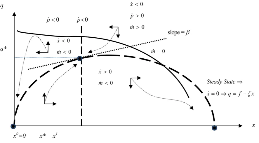
σ < . Again, a saddle point ex-ists and only the nature of the steady-state changes. Now, by Equation (15), the path defined by m =0 gener-ally lies above x=0. Therefore, as the spacial variability of rainfall declines, at the steady-state, the farmer is consolidating his plots

(

m <0

)

. Because weather risk is declining, the benefits accruing to the enforcement of private property rights exceed the benefits of dispersing land into subplots (Figure 2).

In the first equilibrium

(

_q=q0 _{=0 and x=x}0 ₌₀

)

_{, barriers to entry such as high initial costs dissuade the}

farmer from producing. However, as subplot dispersion decreases, costs become less formidable. As a result, in the second equilibrium the farmer chooses to produce and sell q=q*>0 at x=x*. In the final equilibrium, the farmer chooses to produce, but elects to consume all output himself (sells nothing). Much like the case where spacial variability in rainfall increases, the market price is not sufficiently high enough to merit selling at market, but costs are still not so high as to abandon production. To summarize, recall that whenever m >0, one moves closer to a system of common property rights.

As the spacial variability of rainfall increases

(

σ >2 0

)

, subplot dispersion is generally concurrent with rising investment. That is, both rising investment and increased crop dispersion are complementary in that both are used to hedge against weather risk. However, as the spacial variability of rainfall decreases

(

2

)

0

σ < , increased investment is consistent with a decline in subplot dispersion. That is, investment and crop dispersion act as subs-titute hedges when weather risk decreases.

4. Conclusion

[image:11.595.93.537.462.707.2]

This model provides a theoretical justification for evolving property rights regimes by providing a dynamic in-tertemporal model demonstrating how changes in risk associated with weather variability motivate farmers to forego private property rights in favor of common property rights. Existing literature concerning spacial varia-bility of rainfall is predominantly descriptive or empirical. Static models are used to implicitly describe a dy-

236

namic process. We believe that this analysis provides a satisfactory theoretic framework to complement previous work and to help guide future research on the topic.

Specifically, the model considers how production and costs, as well as the benefits of maintaining private property rights, influence property rights regimes when the spacial variability of rainfall is changing over time. Weather risk increases in response to increases in the spacial variability of rainfall. As this risk increases, far-mers are motivated to relinquish control over their property in order to induce neighbors to risk-pool by subdi-viding and sharing land endowments. Specifically, when utility is maximized, an increase in the spacial varia-tion of rainfall leads to a rise in the rate of subplot dispersion. Similarly, when spacial variavaria-tion is constant or falling, farmers are motivated to maintain private property (land endowments).

We demonstrate the existence of three equilibria consistent with intertemporal utility maximization in the face of first increasing and then decreasing, spacial variability of rainfall. In the first equilibrium, the farmer elects to produce nothing because high start-up costs serve as a barrier to entry. In the second equilibrium, the farmer re-duces production risk via plot dispersion. This act of risk-pooling in the face of increasing spacial variability in rainfall decreases risk, allowing the farmer to both consume and to sell portions of his production. In the final equilibrium, further diversification of subplots causes a significant increase in transportation and transactions costs, but farmers continue to produce. Farmers invest more, but consume all that they produce.

We find that as the spacial variability of rainfall increases, subplot dispersion is generally concurrent with rising investment. That is, rising investment and increased crop dispersion are complementary hedges against weather risk. We also describe three similar equilibria that occur when the spacial variability of rainfall is de-clining. However, in this case, as weather risk declines increased investment is consistent with a decline in sub-plot dispersion. That is, investment and crop dispersion act as substitute hedges against weather risk as that risk decreases. This is consistent with the proposition that individuals will move towards a system of private property rights as weather risk declines.

Understanding how property rights regimes can evolve is important when formulating appropriate develop-ment policy. The dissolution of private property rights can radically change the status quo. It can lead to nomad-ic migration whnomad-ich can increase tension among tribal groups, or compromise state or international borders. Also, credit markets typically rely on land as collateral, particularly in developing nations. Increased weather risk that leads to the disbanding of private property rights has the potential to significantly disrupt credit markets. More-over, as weather patterns across the globe change in response to global warming, we should expect more social upheaval and more strain on existing institutions. As a result, more research into the impact of weather risk on property rights and other institutions is needed.

Acknowledgements

F.E.R. wishes to thank Nick Sanchez for calling attention to the need to investigate this problem from a theoreti- cal perspective.

References

[1] Ray, D. (1998) Development Economics. Princeton University Press, Princeton.

[2] Hardin, G. (1968) The Tragedy of the Commons. Science, 162, 1243-1248. http://dx.doi.org/10.1126/science.162.3859.1243

[3] Sethi, R. and Somanathan, E. (1996) The Evolution of Social Norms in Common Property Resource Use. American Economic Review, 86, 766-788.

[4] Levine, R. (1997) Financial Development and Economic Growth: Views and Agenda. Journal of Economic Literature,

35, 688-726.

[5] Coase, R. (1960) The Problem of Social Cost. The Journal of Law and Economics, 3, 1-44. http://dx.doi.org/10.1086/466560

[6] Tornell, A. (1997) Economic Growth and Decline with Endogenous Property Rights. Journal of Economic Growth, 2, 219-250. http://dx.doi.org/10.1023/A:1009749908420

[7] Van Long, N. and Sorger, G. (2006) Insecure Property Rights and Growth: The Role of Appropriations Costs, Wealth Effects and Heterogeneity. Economic Theory, 28, 513-529. http://dx.doi.org/10.1007/s00199-005-0635-4

Lit-237

tlefield, Lanham, 69-83.

[9] Li, T.M. (1996) Images of Community: Discourse and Strategy in Property Relations. Development and Change, 27, 23-51. http://dx.doi.org/10.1111/j.1467-7660.1996.tb00601.x

[10] De Zeeuw, F. (1997) Borrowing of Land, Security of Tenure and Sustainable Land Use in Burkina Faso. Development and Change, 28, 19-41.

[11] Goodhue, R.E. and McCarthy, N. (2009) Traditional Property Rights, Common Property, and Mobility in Semi-Arid African Pastoral Systems. Environment and Development Economics, 14, 29-50.

http://dx.doi.org/10.1017/S1355770X08004555

[12] Tucker, C.M. (2010) Private Goods and Common Property: Pottery Production in a Honduran Lenca Community.

Human Organization, 69, 43-53.

[13] Chiang, S.H. and Li, X. (2010) Market Correlation and Property Rights. Journal of Institutional and Theoretical Eco-nomics, 166, 426-438. http://dx.doi.org/10.1628/093245610793102143

[14] Rosenzweig, M.R. and Binswanger, H.P. (1993) Wealth, Weather Risk and the Consumption and Profitability of Agri- cultural Investments. The Economic Journal, 103, 56-78. http://dx.doi.org/10.2307/2234337

[15] McCloskey, D.N. (1989) The Open Fields of England: Rent, Risk and the Rate of Interest, 1300-1815. In: Galenson, D.W., Ed., Markets in History: Economic Studies of the Past, Cambridge University Press, Cambridge, 5-51.

[16] Nugent, J. and Sanchez, N. (1998) Common Property Rights as an Endogenous Response to Risk. American Journal of Agricultural Economics, 80, 651-657. http://dx.doi.org/10.2307/1244575

[17] Nugent, J. and Sanchez, N. (1999) The Local Variability of Rainfall and Tribal Institutions: The Case of Sudan. Jour-nal of Economic Behavior and Organization, 39, 263-292. http://dx.doi.org/10.1016/S0167-2681(99)00036-0

[18] De Meza, D. and Gould, J.R. (1992) The Social Efficiency of Private Decisions to Enforce Property Rights. Journal of Political Economy, 100, 561-580. http://dx.doi.org/10.1086/261829

[19] Crépin, A. and Lindahl, T. (2009) Grazing Games: Sharing Common Property Resources with Complex Dynamics. En- vironmental and Resource Economics, 44, 29-46. http://dx.doi.org/10.1007/s10640-008-9258-0