www.hydrol-earth-syst-sci.net/12/1121/2008/ © Author(s) 2008. This work is distributed under the Creative Commons Attribution 3.0 License.
Earth System
Sciences
Estimation of streamflow by slope regional dependency function
A. Altunkaynak
Istanbul Technical University, Faculty of Civil Engineering, Maslak 34469, Istanbul, Turkey Received: 20 February 2008 – Published in Hydrol. Earth Syst. Sci. Discuss.: 11 April 2008 Revised: 18 June 2008 – Accepted: 9 July 2008 – Published: 25 August 2008
Abstract. Kriging is one of the most developed
methodolo-gies in the regional variable modeling. However, one of its drawbacks is that the influence radius can not be determined by this method. In which distance and in what ratio that pivot station is influenced from adjacent sites is rather of-ten encountered problem in practical applications. Regional weighting functions obtained from available data consist of several broken lines. Each line has different slopes which represent the similarity and the contribution of adjacent sta-tions as a weighting coefficient. The approach in this study is called as Slope Regional Dependency Function (SRDF). The main idea of this approach is to express the variabil-ity in value differencesγ and distances together. Originally proposed SRDF and Trigonometric Point Cumulative Semi-Variogram (TPCSV) methods are used to predict streamflow. TPCSV and Point Cumulative Semi-Variogram (PCSV) ap-proaches are also compared with each other. Prediction per-formance of all the three methods revealed a relative error less than 10% which is acceptable for most engineering ap-plications. It is shown that SRDF outperforms PCSV and TPCSV with very high differences. It can be used for miss-ing data completion, determination of measurement sites lo-cation, calculation of influence radius, and determination of regional variable potential. The proposed method is applied for the 38 stream flow measurement sites located in the Mis-sissippi River basin.
Correspondence to: A. Altunkaynak ([email protected])
1 Introduction
The quantity of streamflow plays a significant role on plan-ning, management and design of the water resources. Dis-charge is directly related with reservoir operation, forecast-ing of floods and droughts, hydroelectric power produc-tion, irrigaproduc-tion, protection of ecosystem and sedimentation. Therefore, prediction and calculation of the discharge are very important.
18 7362000 0 0,1 0,2 0,3 0,4 0,5 0,6 0,7 0,8 0,9 1
0,00 0,10 0,20 0,30 0,40 0,50 0,60 0,70 0,80 0,90 1,00
[image:2.595.50.284.63.199.2]Standard distance S tandard P C S V Regional Weighting Function Figure 1.
α Δγi
Δdi
0
Regional dependency function PCSV
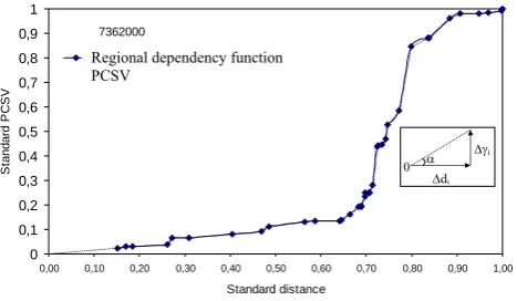
Fig. 1. Regional Dependency Function according to PCSV.
Peng and Buras (2000) used spatial method to esti-mate discharge for multi-reservoir operation. In case of non-stationarity and irregularity of measurement points, S¸en (1989) proposed Point Cumulative Semi Variogram (PCSV) approach based on relationship between point and area. It is possible to determine influence radius from se-lected point by standard regional dependence procedure in-troduced by S¸en and Habib (1998). To determine the ef-fective range and weighting coefficient of a variable is very important for estimations and calculations. PCSV method is based on the differences between selected pivot point and the surrounding points. The recorded variables in the points constitute differences that lead to regional dependence func-tions. These functions can be used for missing data comple-tion, optimum location of measurement sites, calculation of influence radius and determination of regional variable po-tential. S¸ahin and S¸en (2004) developed Trigonometric Point Cumulative Semi Variogram (TPCSV) technique and applied to wind data. Also, Altunkaynak (2005) applied this method for the estimation of ocean wave characteristics.
The aim of the study is to estimate the station values from neighboring stations by using Slope Regional Dependency Function (SRDF). The proposed method is applied for the stream flow measurement network located in the Mississippi River basin.
2 Regional Dependency Function (RDF)
PCSV method is based on the half square differences [γ (d)] between pivot site and randomly scattered adjacent sites. This approach searches the effect of one point to the other points. It is possible to obtain data of stations which are not measured or missing by using regional weighting functions. Moreover, influence radius of each site can be determined by these functions. If the difference is very high between two stations then the next station would not be taken into consid-eration in calculations. The relationship between points can
7362000 0 0.1 0.2 0.3 0.4 0.5 0.6 0.7 0.8 0.9 1 1.1 1.2 1.3 1.4 1.5 Regional dependency function TPCSV
cos(
α
)
0.00 0.10 0.20 0.30 0.40 0.50 0.60 0.70 0.80 0.90 1.00
[image:2.595.309.544.64.203.2]Standard distance
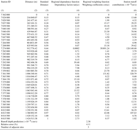
Fig. 2. Regional Dependency Function according to TPCSV.
be given as following equation. γ (di)=
1
2 qp−qdi
2
(i=1,2,· · ·n) (1)
Whereqpandqd are pilot station and adjacent stations
dis-charge values, respectively. n is the number of stations. When it is desired to show the variation of PCSV values by distance on a Cartesian coordinate system, the x-axis rep-resents the distances from pivot point and the y-axis repre-sents the PCSV values. For the sake of simplicity, Eq. (1) should be standardized. After this operation, x- and y-axes take the values ranging from 0 to 1. Standardization can be achieved by dividing the all values to the maximum. It can be said that as the distance increases the correlation between pivot and other points decreases and also the weighting co-efficient which represents the contribution of adjacent points decreases. The weightings of the highly correlated points approach to 1. On the other hand it takes 0 for uncorrelated points.
S¸ahin ve S¸en (2004) applied TPCSV technique to the wind data. This approach was also developed by considering cor-relation principle. Two different data array can be put in the same set when they are highly correlated. Two data array,
x=(a11, a12, a13,· · ·a1n)andy=(a21, a22, a23,· · ·a2n)are
the vectors which have the same initial point. The angle be-tween two vectors is required for determination of similarity of two data arrays or vectors. Scalar multiplication ofxand
yvectors is indicated as below. cosα=
* x· * y *x · * y (2)
As the angle is narrower, these two points or arrays show more similarity. If the angle is zero, it can be said that there is an exact dependency between these points or arrays and the correlation coefficient is equal to 1. In contrast, if the angle is 90◦two points or arrays have no dependency and the cor-relation coefficient is equal zero. Consequently as the angle increases, the similarity reduces. The regional dependence function depicted in Fig. 1 shows cosα values of stations found in thed distance from pivot point and contributions of these points to pivot point. The point selected in the figure is shown as,
1di=di+1−di, (3)
where1dis the distance difference between two consecutive points. Theγ (d) between two consecutive points on y-axis of the same figure is shown as1γ.
1γi=γ (di+1)−γ (di) (4)
Hypotenuse value is required to determine the value of cosα. The square root of summation squares of Eqs. (3) and (4) give hypotenuse.
|AB|i=
q
(1di)2+(1γi)2 (5)
|AB| is the length of the line which is constituted by two points. All cosαvalues in the same figure can be calculated as following.
(cosαi)i=
1di
|AB|i (6)
The number of cosα value calculated is n-1 which corre-sponds to n points. The angle range is from 0◦ to 90◦,
because regional dependency function increases monotony. The weighted average is used in the prediction of pivot sta-tion discharge value. The summasta-tion of cosαvalues is,
L=cosα1+cosα2+· · ·cosαn. (7)
WhereLis sum of the cosαvalues. Following expression is given for the prediction of pivot point value.
qp=
1 L
N X
i=1
qi ·cosαi (8)
Here cosα is expressed as the weighting coefficient. The regional dependency function shown in Fig. 1 increases con-tinuously by the distance. Function curve exhibits distinct features in different portions of distances such as it rise more linearly, increasingly or decreasingly. Regional dependency function consists of several lines. Slope of the each line (tanα) explains the similarity between two points. It also gives information about the regional dependency. The ra-tio of the γ (d)differences, 1γ (d) to distance differences leads to slope which is the first derivation of line. If the dif-ferences between the points are small then this means that
the slope will reduce and dependency will increase. On con-trary, steep slope means weak dependency. Bothγ (d)and distance variations are taken into account together by consid-ering the slope regional dependency function (SRDF) which is the main idea of this study. Closeness to pivot point does not mean that they are very similar to each other and their correlation is high. The square of differences(qp−qd)2
be-tween pivot point and close points should be low. Hereqp
andqd are the runoff depths at pivot point and the point at
d distance, respectively. When distance andγ (d)variations are low, it can be said that these two points are very similar and their contribution to value of pivot point prediction are very high. The effect of bothγ (d)differences,1γ (d)and the distance differences between two points,1d, is consid-ered together in this approach. The ratio of 1γ (d)to1d gives dimensionless slope.
Dependency factor=tanα=1γ (d)
1d (9)
when tanαvalue between two points is lower, it contributes more to the weighting average of pivot point. Therefore, re-gional dependency function slope identified as dependency factor of this point. The slope (tanα) of regional dependency function gives the similarity and dependency. The flatter slope contributes to pivot point with high weighting coeffi-cient. In contrast, the contribution of point to the pivot point is very low when the slope is very steep. There is an inverse relationship between slope and adjacent sites contribution. The weighting coefficient that represents the contribution of a point is equal to cotα.
Weighting coefficient=cotαi=
1d
1γ (d) (10)
cotαis used instead of cosαwhich is employed for TPCSV method for prediction of the pivot point value. The sum-mation of cotαvalues used in weighted average is given as below.
m=cotα1+cotα2+ · · ·cotαn (11)
Here mis the summation of weighting coefficients. cosα in Eq. (8) used for TPCSV method is replaced by cotα to predict the pivot point discharge value.
qp=
1 m
Nd
X
i=1
qi·cotαi (12)
Here,qpis runoff depth value of the predicted pivot point.
Table 1. Station 7 362 000 Detailed Prediction Calculations According to SRDF.
Station ID Distance (m) Standard Regional dependency function Regional weighting function Station runoff
Distance Dependency factors tan(α) Weighting coefficients cot(α) contributions×10−8(m/s)
(1) (2) (3) (4) (5) (6)
7 362 000 0 0 0 0 0
7 024 000 216 840.07 0.15 0.15 6.90 13.68
7 029 500 241 477.41 0.17 0.50 1.99 4.32
7 037 500 263 101.21 0.18 0.07 15.17 39.25
7 039 500 371 389.53 0.26 0.10 10.18 22.30
7 040 100 388 591.64 0.27 2.11 0.47 0.92
7 040 450 439 964.87 0.31 0.03 33.30 78.96
7 043 500 575 431.33 0.40 0.14 7.12 14.92
7 047 900 667 068.52 0.47 0.22 4.50 9.36
7 077 500 692 493.58 0.49 0.93 1.07 2.19
7 264 000 80 4831.69 0.56 0.28 3.52 6.98
7 268 000 835 993.04 0.59 0.07 15.18 39.62
7 274 000 912 776.42 0.64 0.0002 50 891.24 126 140.68
7 282 000 919 920.48 0.65 0.71 1.41 3.79
7 283 000 945 863.96 0.66 1.32 0.76 2.27
7 290 000 971 207.44 0.68 1.70 0.59 1.12
7 291 000 982 319.79 0.69 0.15 6.77 17.57
7 292 500 982 406.38 0.69 59.48 0.02 0.05
7 295 000 991 568.73 0.70 5.94 0.17 0.53
7 356 000 994 219.29 0.70 7.98 0.13 0.36
7 359 002 1 003 885.50 0.70 0.04 23.70 60.16
7 361 500 1 006 340.44 0.71 0.01 131.82 328.79
7 363 500 1 016 046.47 0.71 4.48 0.22 0.68
7 364 150 1 031 071.40 0.72 15.10 0.07 0.25
7 375 000 1 034 253.36 0.73 0.70 1.42 3.72
7 375 500 1 045 620.01 0.73 0.38 2.63 7.02
7 376 000 1 057 498.31 0.74 2.89 0.35 0.68
7 376 500 1 063 043.46 0.75 15.52 0.06 0.21
7 377 500 1 098 912.20 0.77 2.27 0.44 0.74
7 378 000 1 136 730.09 0.80 9.79 0.10 0.08
7 378 500 1 191 312.39 0.84 0.93 1.08 3.36
7 382 500 1 195 026.19 0.84 0.20 5.12 12.31
7 385 500 1 259 797.11 0.88 1.78 0.56 1.93
8 010 000 1 292 656.90 0.91 0.71 1.41 4.10
8 012 000 1 350 351.98 0.95 0.07 13.61 36.29
8 013 500 1 380 892.95 0.97 0.02 42.08 107.63
8 014 500 1 420 152.16 1.00 0.32 3.12 6.76
8 015 500 1 424 513.38 1 2.73 0.37 1.02
Runoff depth prediction (×10−8) (m/s) 2.38
Relative error (%) 4.11
Number of adjacent sites 3
3 Application
In this study, 38 measurement stations located in Mississippi River basin are used. Data is obtained from the study of Al-tunkaynak et al. (2005). The aim of using the same data is to compare PCSV, TPCSV and SRDF methods under equal conditions. Altunkaynak et al. (2005) computed runoff depth values of 38 measurement stations by using PCSV technique. Here, TPCSV and proposed model are employed for the same data. Study area, location map and detailed informa-tion on PCSV technique can be found in the study of Al-tunkaynak et al. (2005). In SRDF method, and for the pivot
20
7362000
0 5 10 15 20 25 30
0.00 0.10 0.20 0.30 0.40 0.50 0.60 0.70 0.80 0.90 1.00
Standard distance
ta
n(α
)
Regional dependency function SRDF
[image:5.595.51.284.55.191.2]Figure 3.
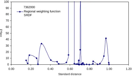
Fig. 3. Regional Dependency Function according to SRDF.
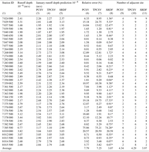
In the second part, it is between 0.7 and 0.8, and increment is seen. Finally in the last part there is a decreasing trend. There is linear trend in the first part, because the slope ap-proaches to a constant value or it fluctuates around a constant value. When one looks at the part of the dependency func-tion which corresponds to 0–0.7 standard distance at hori-zontal axis in Fig. 3, low fluctuations of tanα=dependency function around a mean value can be seen.On the other hand, there is an agreement with the weighting coefficient which corresponds to same range in Fig. 4. Also, it can be said that this region exhibits a homogeny structure. The expres-sion of homogeny structure means that stations found in this region are similar to each other and have strong regional de-pendency. The increasing rise of regional weighting func-tion in Fig. 1 corresponds to a porfunc-tion (0.7–0.8) which has big fluctuations in Fig. 3. There is heterogenic structure in this part. The stations found in this region have no similar-ities and dependencies with pivot station. Although there is a decreasing rise trend in the third portion of Fig. 1, devia-tions from the mean are less than second portion shown in Figs. 3 and 4. The similarities and correlations to pivot sta-tion in this part are more than the second part. Mississippi River Basin can be divided into three part based on regional weighting function. Since the second part has high hetero-geneity, it can be divided into more sub regions. This can be an input for the integrated basin management. Figs. 1, 3 and 4 demonstrate that which distances are homogeny or hetero-genic in the first, second and third parts.The influence radius can be determined by this way. All these interpretations can be made by using Fig. 2 that shows the dependency func-tion. Also, three parts are seen obviously from this figure too. Low deviations from the mean value at 0–0.7 standard distance, high variability of dependency at 0.7–0.8 and lower variation of dependency comparing to second part at 0.8–1.0 are also valid in this figure. It is possible to predict missing or unmeasured runoff depths by using these functions. Let it is assumed that runoff depth data for the station 7 362 000 is unavailable or missing.
21
7362000
0 10 20 30 40 50 60 70 80 90 100
0.00 0.20 0.40 0.60 0.80 1.00 1.20
Standard distance
co
t(
α
)
Regional weighting function SRDF
[image:5.595.312.545.61.194.2]Figure 4.
Fig. 4. Regional Weighting Function according to SRDF.
Table 2. Comparison of PCVS, TPCVS and SRDF methods.
Station ID Runoff depth January runoff depth prediction 10−8 Relative error (%) Number of adjacent site 10−8(m/s) (m/s)
PCSV TPCSV SRDF PCSV TPCSV SRDF PCSV TPCSV SRDF
(1) (2) (3) (4) (5) (6) (7) (8) (9) (10) (11)
7 024 000 2.41 2.26 2.27 2.37 6.33 8.95 1.36* 4 9 9
7 029 500 3.31 2.81 2.48 3.13 15.18 24.75 5.33* 2 9 2
7 037 500 1.68 1.95 1.92 1.91 14.04 13.02 12.47* 3 2 2
7 039 500 1.96 1.99 1.98 1.97 1.65 1.20 0.81* 4 4 3
7 040 100 1.90 1.87 1.87 1.95 1.72 1.30 2.75 3 3 3
7 040 450 1.98 2.01 2.00 1.97 1.63 1.39 0.46* 3 3 5
7 043 500 2.05 2.05 2.05 2.04 0.01 0.14 0.38 5 3 3
7 047 900 2.08 2.04 2.08 2.09 1.58 0.09 0.54* 5 4 3
7 077 500 2.09 2.11 2.10 2.08 0.52 0.61 0.67 3 3 2
7 264 000 2.19 2.19 2.18 2.14 0.01 0.55 2.05 4 4 7
7 268 000 3.14 2.73 2.73 3.08 12.89 12.81 1.72* 4 4 4
7 274 000 2.48 2.49 2.61 2.53 0.44 5.12 2.23 9 6 5
7 282 000 2.54 2.54 2.54 2.53 0.01 0.06 0.02 8 2 9
7 283 000 2.60 2.59 2.60 2.60 0.01 0.16 0.46 7 8 5
7 290 000 2.61 2.60 2.66 2.61 0.42 2.06 0.21* 7 3 2
7 291 000 2.62 2.78 2.69 2.61 5.91 2.82 0.23* 4 2 4
7 292 500 2.49 2.76 2.74 2.64 9.52 9.21 5.67* 2 2 2
7 295 000 2.89 2.88 2.87 2.91 0.38 0.55 0.68 6 6 3
7 356 000 2.37 2.42 2.38 2.37 1.81 0.20 0.04* 3 2 7
7 359 002 2.59 2.31 2.32 2.34 10.97 10.38 9.38* 4 4 4
7 361 500 2.17 2.33 2.26 2.19 7.04 3.98 1.12* 5 6 4
7 362 000 2.48 2.24 2.25 2.38 9.69 9.33 4.11* 3 3 3
7 363 500 1.98 2.20 2.20 1.95 9.95 9.90 1.61* 8 3 3
7 364 150 1.95 2.14 2.14 1.98 9.18 9.36 2.01* 6 6 2
7 375 000 2.17 2.68 2.70 2.60 19.18 19.75 17.33* 3 9 2
7 375 500 2.79 3.17 2.78 2.76 12.07 0.27 0.91* 2 6 7
7 376 000 2.67 2.76 2.73 2.64 3.17 2.49 0.8* 3 2 4
7 376 500 2.56 2.54 2.57 2.65 1.28 0.68 3.62 3 3 3
7 377 500 3.12 2.54 3.17 3.11 18.60 1.91 0.1* 3 2 3
7 378 000 3.44 3.02 3.01 3.07 12.10 12.26 10.7* 2 2 2
7 378 500 2.91 2.92 2.90 2.83 0.37 0.30 2.53 5 4 8
7 382 500 2.67 2.65 2.81 2.68 0.82 5.29 0.75* 7 6 5
7 385 500 0.77 3.17 3.10 2.99 75.86 75.21 74.28* 6 2 2
8 010 000 3.82 3.04 3.03 3.03 20.57 20.59 20.59 2 2 2
8 012 000 3.07 3.05 3.05 3.05 0.71 0.50 0.55* 4 4 8
8 013 500 3.00 2.99 2.97 3.01 0.73 0.93 0.35* 5 4 5
8 014 500 2.68 2.79 2.78 2.68 3.92 3.68 0.07* 6 8 2
8 015 500 2.68 2.84 2.79 2.68 5.77 3.82 0.07* 2 8 2
Average 7.79 7.25 3.07 4.34 4.29 3.97
SRDF predicts 26 out of 38 stations value more accu-rate than TPCSV. The mean relative errors for the SRDF and TPCSV are 3.07% and 7.25%, respectively. The num-ber of stations which has relative errors less than 10% is 5 and 8 for the SRDF and TPCSV, respectively. After all, it is evident that PCSV and TPCSV performances are close to each other. The relative error is 7.79% for PCSV and 7.25% for the TPCSV. There is not a huge difference between two methods. However, SRDF substantially outperforms PCSV and TPCSV techniques which can be seen from Table 2.
4 Conclusions
In this study, 38 runoff measurement sites located in the Mis-sissippi River Basin are used for the implementation of pro-posed method. The regional dependency function for each station is calculated. Regional dependency functions are obtained by TPCSV method and dependency and weight-ing functions are obtained by SRDF. Runoff predictions are made by using SRDF and TPCSV methods for all stations. Each station influence of radius is determined. Regional de-pendency function is obtained from available data. In 28 and 26 among 38 stations, the proposed approach SRDF has lower relative error than PCSV and TPCSV techniques, re-spectively. PCSV and TPCSV show nearly the same pre-diction performances. The mean relative errors for all three methods are less than 10% which are acceptable in engineer-ing applications. The graphical and numerical criteria are employed to show the better performance of SRDF against PCSV and TPCSV. All results in the tables are interpreted and compared with each other.
Edited by: A. Shamseldin
References
Altunkaynak, A.: Significant wave height prediction by using a spa-tial model, Ocean. Eng., 32(8–9), 924–936, 2005.
Altunkaynak, A. and ¨Ozger, M.: Spatial significant wave height variation assessment and its estimation, J. Waterw. Port C.-ASCE, 131(6), 277–282, 2005.
Altunkaynak, A., ¨Ozger, M., and Sen, Z.: Regional stream flow estimation by Standard regional dependence function approach, J. Hydraul. Eng.-ASCE, 131(11), 1001–1006, 2005.
Altunkaynak, A., ¨Ozger, M., and S¸en, Z.: Triple diagram model of level fluctuations in Lake Van, Turkey, Hydrol. Earth Syst. Sci., 7, 235–244, 2003,
http://www.hydrol-earth-syst-sci.net/7/235/2003/.
Huang, W. C. and Yang, F. T.: Streamflow estimation by using Krig-ing, Water Resour. Res., 34(6), 1599–1608, 1998.
Krige, D. G.: A statistical approach to some basic mine valuation problems on the Witwatersrand, J. Chem. Metall. Min. Soc. S. Afr., 52, 119-139, 1951.
Matheron, G.: Principles of geostastistics, Econ. Geol., 58, 1246– 1266, 1963.
Matheron, G.: The theory of regionalized variables and Its applica-tions, Ecole de Mines, Fontainbleau, France, 1971.
Matias, J. M., Vaamondel, A., Taboada, J., and Gonzalez-Manteiga, W.: Comparison of Kriging and neural networks with application to the exploitation of a slate mine, Math. Geol., 36(4), 463–486, 2004.
Peng, C. S. and Buras, N.: Practical estimation of inflows into mul-tireservoir system, J. Water Res. Pl.-ASCE, 126(5), 331–334, 2000.
¨
Ozt¨urk, C. A. and Nasuf, E.: Geostatistical assessment of rock zones for tunneling, Tunnelling and Underground Space Tech-nology, 17(3) , 275–285, 2002.
S¸ahin, A. D. and S¸en, Z.: A new spatial prediction model and its application to wind records, Theor. Appl. Climatol., 79(1–2), 45– 54, 2004.
S¸en, Z. and Habib, Z. Z.: Point cumulative semivariogram of areal precipitation in mountainous regions, J. Hydrol., 205, 81–91, 1998.