www.hydrol-earth-syst-sci.net/21/1077/2017/ doi:10.5194/hess-21-1077-2017
© Author(s) 2017. CC Attribution 3.0 License.
Geostatistical upscaling of rain gauge data to support uncertainty
analysis of lumped urban hydrological models
Manoranjan Muthusamy1, Alma Schellart1, Simon Tait1, and Gerard B. M. Heuvelink2 1Department of Civil and Structural Engineering, University of Sheffield, Sheffield, S1 3JD, UK 2Soil Geography and Landscape group, Wageningen University, Wageningen, 6700, the Netherlands
Correspondence to:Manoranjan Muthusamy ([email protected]) Received: 31 May 2016 – Discussion started: 20 June 2016
Revised: 4 December 2016 – Accepted: 13 January 2017 – Published: 20 February 2017
Abstract.In this study we develop a method to estimate the spatially averaged rainfall intensity together with associated level of uncertainty using geostatistical upscaling. Rainfall data collected from a cluster of eight paired rain gauges in a 400 m×200 m urban catchment are used in combination with spatial stochastic simulation to obtain optimal predic-tions of the spatially averaged rainfall intensity at any point in time within the urban catchment. The uncertainty in the prediction of catchment average rainfall intensity is obtained for multiple combinations of intensity ranges and temporal averaging intervals. The two main challenges addressed in this study are scarcity of rainfall measurement locations and non-normality of rainfall data, both of which need to be con-sidered when adopting a geostatistical approach. Scarcity of measurement points is dealt with by pooling sample vari-ograms of repeated rainfall measurements with similar char-acteristics. Normality of rainfall data is achieved through the use of normal score transformation. Geostatistical models in the form of variograms are derived for transformed rainfall intensity. Next spatial stochastic simulation which is robust to nonlinear data transformation is applied to produce real-isations of rainfall fields. These realreal-isations in transformed space are first back-transformed and next spatially aggre-gated to derive a random sample of the spatially averaged rainfall intensity. Results show that the prediction uncertainty comes mainly from two sources: spatial variability of rainfall and measurement error. At smaller temporal averaging inter-vals both these effects are high, resulting in a relatively high uncertainty in prediction. With longer temporal averaging in-tervals the uncertainty becomes lower due to stronger spatial correlation of rainfall data and relatively smaller measure-ment error. Results also show that the measuremeasure-ment error
in-creases with decreasing rainfall intensity resulting in a higher uncertainty at lower intensities. Results from this study can be used for uncertainty analyses of hydrologic and hydrody-namic modelling of similar-sized urban catchments as it pro-vides information on uncertainty associated with rainfall es-timation, which is arguably the most important input in these models. This will help to better interpret model results and avoid false calibration and force-fitting of model parameters.
1 Introduction
spa-tial correlation structure of the rainfall and the spaspa-tial organ-isation of the rain gauge locations. Another commonly used method in hydrological modelling is the nearest neighbour interpolation (Chow, 1964; Nalder and Wein, 1998) which leads to Thiessen polygons. In this method the nearest ob-servation is given a weight of one and other obob-servations are given zero weights during interpolation, thereby ignoring spatial variability of rainfall to a certain extent. There are also other methods, with varying complexity levels, including verse distance weighting (Dirks et al., 1998), polynomial in-terpolation (Tabios III and Salas, 1985) and moving window regression (Lloyd, 2005). The predictive performance of the above methods are found to be case dependent and no single method has been shown to be optimal for all catchments and rainfall conditions (Ly et al., 2013). One common drawback with all the above methods is that they do not provide any in-formation on the uncertainty of the predictions of AARI as all the methods are deterministic. The uncertainty in prediction of AARI mainly comes from two sources; uncertainty due to measurement errors and uncertainty associated with spatial variability of rainfall. The characteristics of measurement er-rors can vary depending on the rain gauge type. For example, errors associated with commonly used tipping bucket rain gauges range from errors due to wind, wetting, evaporation, and splashing (Fankhauser, 1998; Sevruk and Hamon, 1984) to errors due to its sampling mechanism (Habib et al., 2001). In addition to measurement errors and since rainfall can vary over space significantly, any spatial aggregation method for scaling up the point rainfall measurements incorporates more uncertainty (Villarini et al., 2008). The magnitude of the un-certainty depends on many factors including rain gauge den-sity and location, rainfall variability, catchment size, topog-raphy, and the spatial interpolation technique used. Quantifi-cation of the level of uncertainty is essential for robust in-terpretation of hydrological model outputs. For instance, the absence of information on uncertainty can lead to force fit-ting of hydrological model parameters to compensate for the uncertainty in rainfall input data (Schuurmans and Bierkens, 2007).
Geostatistical methods such as kriging present a solution to this problem by providing a measure of prediction er-ror. In addition to this capability, these statistical methods also take into account the spatial dependence structure of the measured rainfall data (Ly et al., 2013; Mair and Fares, 2011). Although these features make geostatistical methods more attractive than deterministic methods, they are rarely used in LCMs due to their inherent complexity and heavy data requirements. Since they are statistical methods encom-passing multiple parameters the amount of spatial data re-quired for model inference is higher compared to determin-istic methods. In addition the underlying assumption of geo-statistical approaches typically requires data to be normally distributed (Isaaks and Srivastava, 1989). In general, catch-ments, especially those at small urban scales, do not contain as many measurement locations as required by
geostatisti-cal methods. Furthermore, rainfall intensity data are almost never normally distributed, especially at smaller averaging intervals (< 1 h) (Glasbey and Nevison, 1997). Despite these challenges geostatistical methods can provide information on uncertainty associated with predicted AARI. This capabil-ity can be utilised in uncertainty propagation analysis in hy-drological models. In literature, geostatistical methods have been used to analyse the spatial correlation structure of rain-fall at various spatial scales (Berne et al., 2004; Ciach and Krajewski, 2006; Emmanuel et al., 2012; Jaffrain and Berne, 2012), however its application to support uncertainty analy-ses of upscaling rainfall data has not been explored.
In this paper we present a geostatistical approach to derive AARI and the level of uncertainty associated with it from observations obtained from multiple “paired” rain gauges lo-cated in a small urban catchment. The proposed approach presents solutions to the above-described challenges of geo-statistical methods. First, it uses pooling of sample vari-ograms of rainfall measurements at different times but with similar characteristics to increase the number of paired ob-servations used to fit variogram models. Second, a data trans-formation method is employed to transform the rainfall data to obtain a normally distributed data set. The level of uncer-tainty in the prediction of AARI is then quantified for differ-ent combinations of temporal averaging intervals and inten-sity ranges for the studied urban catchment. We focused on a small urban catchment with a spatial extent of less than a kilometre given the findings of recent research on the high significance of unmeasured spatial rainfall variability at such spatial scales, especially for urban hydrological and hydro-dynamic modelling applications (Gires et al., 2012, 2014; Ochoa-Rodriguez et al., 2015).
2 Data collection
2.1 Location and rain gauge network design
surround-Figure 1.Left: aerial view of rain gauge network covering an area of 400 m×200 m at Bradford University, UK. Right: a photograph of paired rain gauges at station 6.
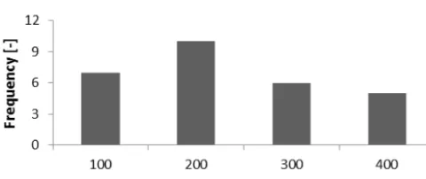
Figure 2. Histogram with class interval width of 100 m showing frequency distribution of inter-station distances (m).
ing ground level following UK standard practice (MetOf-fice UK, 2016). An example of the measurement setup (sta-tion 6) is also shown in Fig. 1. A histogram of the inter-station distances of the rain gauge network is presented in Fig. 2. Lag distances covered in this network are distributed between 21 m (stations 4–5) and 399 m (stations 1–3).
All rain gauges are ARG100 tipping bucket type with an orifice diameter of 254 mm and a resolution of 0.2 mm. Dy-namic calibration was carried out for each individual gauge before deployment and visual checks were carried out every 4–5 weeks during the measurement period to ensure that the instruments were free of dirt and debris. Data loggers were reset every 4–5 weeks during data collection to avoid any significant time drift. Measurements (number of tips) were taken every minute and recorded on TinyTag data loggers mounted in each rain gauge.
Quality control procedures were performed prior to sta-tistical analysis, taking advantage of the paired gauge setup to detect gross measurement errors. The paired gauge de-sign provides efficient quality control of the rain gauge data records as it helps to identify the instances when one of the
gauges fails, and to clearly identify periods of missing or incorrect data (Ciach and Krajewski, 2006). During the dy-namic calibration of all rain gauges in the laboratory before deployment, it was identified that the highest and lowest val-ues of the calibration factors for the tipping bucket size are 0.196 and 0.204 mm. The gauges were recalibrated in the lab-oratory after the first period of measurement and it was found that the largest change in calibration factor for any gauge was a maximum of 4 % of the original calibration factor. There-fore a maximum difference of 4 % in volume per tip was as-sumed to be caused by inherent instrument error. It was there-fore decided that this is the maximum acceptable difference between any pair of gauges. Sets of cumulative rainfall data corresponding to specific events from the paired gauges were checked against each other and if the (absolute) difference in cumulative rainfall was greater than 4 %, that complete set was identified as unreliable and removed from further analy-sis.
2.2 Characteristics of the data
[image:3.612.49.289.311.412.2]Figure 3.Time series of network average daily rainfall in the two seasons of 2012 and 2013 with vertical dashed lines indicating the events presented in Table 1.
The data set for 2012 and 2013 contains 13 events yield-ing more than 10 mm network average rainfall depth each and lasting for more than 20 min. A summary of these events is presented in Table 1. Note that this event separation is only used for the presentation of results in Sect. 4.2. Hence it does not leave out any data from the development and cal-ibration of the geostatistical model as presented in Sect. 3. Table 1 shows that the total event duration ranges from 1.5 to 11.4 h while the event network average rainfall intensity varies from 1.79 to 7.96 mm h−1. Table 1 also includes sum-mary statistics of peaks of events (temporal averaging inter-val of 5 min) for the eight stations within the network. Al-though the spatial extent of the area is only 400 m×200 m, it is clear that there is a considerable difference in rainfall in-tensity measurements indicated by the standard deviation and range of peaks observed in the individual events. The maxi-mum standard deviation between peaks of individual events is 9.27 mm h−1for event 8, which is around 12.5 % of the mean network peak intensity of 74.4 mm h−1. This variation provides evidence of the potential importance of analysing uncertainty in the estimation of AARI even in such a small urban catchment.
3 Methodology
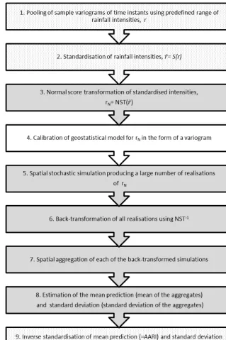
Figure 4 summarises the procedure of geostatistical upscal-ing of the rainfall data adapted in this study in a step-by-step instruction followed by the detail descriptions of each step. This complete procedure was repeated for temporal averag-ing intervals of 2, 5, 15, and 30 min in order to investigate the effect of temporal aggregation on the prediction of AARI.
The entire 10 months of collected data were used for the de-velopment and calibration of the geostatistical model. 3.1 Step 1: pooling of sample variograms
The rain gauge network contains eight measurement loca-tions. These eight measurement locations give 28 spatial pairs at a given time instant which yields too few spatial lags than would normally be used in geostatistical modelling. For example, Webster and Oliver (2007) recommend around 100 measurement points to calibrate a geostatistical model. The procedure adapted in this study increases the number of pairs by pooling sample variograms for time instants with similar rainfall characteristics. With n measurement loca-tions and measurements taken att time instants, the pool-ing overt time instants createst×1/2×n×(n−1) spatial pairs. Although this procedure increases the number of spa-tial pairs by a factor t, the spatial separation distances for which information is available will be limited to the original configuration of thenmeasurement locations.
Table 1.Summary of events which yielded more than 10 mm rainfall and lasted for more than 20 min with summary statistics of event peaks (derived at 5 min temporal averaging interval) from all stations.
Event Date Network Network Network Summary statistics of ID average average average peaks between different
duration intensity rainfall stations (mm h−1)
(h) (mm h−1) (mm) Mean SD Max Min
1 18/04/2012 6.33 2.20 13.9 5.10 0.550 6.02 4.74 2 25/04/2012 6.42 2.55 16.3 7.05 0.751 8.32 5.92 3 09/05/2012 8.92 1.79 16.0 5.10 0.537 5.97 4.74 4 14/06/2012 6.83 1.99 13.6 5.25 0.636 6.04 4.74 5 22/06/2012 11.4 2.39 27.3 12.7 1.72 15.4 9.67 6 06/07/2012 4.42 5.31 23.4 38.5 4.52 42.9 30.5 7 06/07/2012 3.25 3.23 10.5 7.20 0.679 8.46 5.93 8 07/07/2012 1.50 7.84 11.8 74.4 9.27 86.5 61.9 9 19/07/2012 3.08 3.35 10.3 12.7 2.01 14.5 9.74 10 15/08/2012 2.00 7.96 15.9 43.0 3.69 47.8 37.5 11 14/05/2013 7.92 2.14 17.0 8.08 1.20 9.55 6.09 12 23/07/2013 1.75 6.51 11.4 37.7 2.09 42.6 35.7 13 27/07/2013 8.17 4.34 35.5 26.6 1.23 27.5 23.8
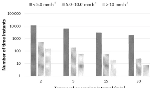
averaging intervals longer than 30 min would not be sensi-ble. Note that although there are only seven time instants, the pooling procedure will produce 196 (=7×28) points to cal-culate and calibrate the geostatistical model for that intensity class.
3.2 Step 2: standardisation of rainfall intensities Having chosen the rainfall intensity classes to create pooled time instants, there can still be inconsistency in spatial vari-ability between time instants within a class and therefore as-suming a single geostatistical model for the whole subset may not be realistic. To reduce this effect to a certain extent, all observations within an intensity class were standardised using the mean and standard deviation of each time instant as follows:
erix=
rix−mi
SDi , (1)
wherei=1 . . .t,x=1 . . .n;erix is standardised rainfall in-tensity at a time instantiand locationx;rixis rainfall inten-sity at time instant iand locationx; andmi, SDi are mean and standard deviation of rainfall intensities at time instanti, respectively. Further steps were carried out on the standard-ised rainfall intensity.
3.3 Step 3: normal transformation of data
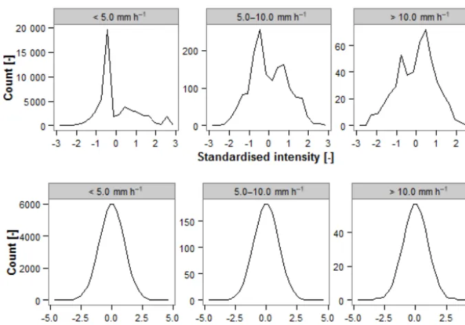
The upper part of Fig. 6 shows the distribution of standard-ised rainfall intensity for a temporal averaging interval of 5 min derived using Eq. (1). From the figure it is clear that the data are not normally distributed. Distributions for other temporal averaging intervals (i.e. 2, 15, and 30 min) show a similar behaviour. But the geostatistical upscaling method to
be used is based on the normal distribution. This requires the rainfall data to be normally distributed prior to the calibration of the geostatistical model. The normal score transformation (NST, also known as normal quantile transformation; Van der Waerden, 1952) is a widely used method to transform a vari-able distribution to the Gaussian distribution. It has widely been applied in many hydrological applications (Bogner et al., 2012; Montanari and Brath, 2004; Todini, 2008; Weerts et al., 2011). The concept of NST is to match thepquantile of the data distribution with thepquantile of the standard nor-mal distribution. Consider a standardised rainfall intensityer with cumulative distributionF
e
R(er) . It is transformed to a rN value with a Gaussian cumulative distributionFRN(rN)
as follows: rN=FR−N1 FRe(er)
. (2)
Detailed description of NST including the steps involved can be found in Bogner et al. (2012), Van der Waerden (1952) and Weerts et al. (2011). The lower part of Fig. 6 shows the transformed standardised intensity for the temporal averag-ing interval of 5 min.
3.4 Step 4: calibration of geostatistical model
Figure 4. Step-by-step procedure developed in this study to predict AARI and associated level of uncertainty. Boxes highlighted in dots indicate the steps to resolve the problem of scarcity in measurement locations, grey boxes show the steps introduced to address non-normality of rainfall data.
depend on explanatory variables (e.g. topography of the area, wind direction). The stochastic termεis spatially correlated and characterised by a variogram model. A variogram model typically consists of three parameters; nugget, sill, and range (Isaaks and Srivastava, 1989). The nugget is the value of the semi-variance at near-zero distance. It is often greater than zero because of random measurement error and micro-scale spatial variation. The range is the distance beyond which the data are no longer spatially correlated. The sill is the
Figure 5.Number of time instants for each temporal averaging in-terval and rainfall intensity class combination.
3.5 Step 5: spatial stochastic simulation
The assumption of a constant trend makes that the spatial interpolation can be solved using an ordinary kriging system (Isaaks and Srivastava, 1989):
n X
y=1
wyγxy−µ=γxz∀x=1, . . ., n (4) n
X
x=1
wx=1, (5)
wherewx,x=1, . . ., nare ordinary kriging weights,γxy is the semivariance between rainfall intensities at locations x andy,γxzis the semivariance between rainfall intensities at locationyand prediction locationz, andµis a Lagrange pa-rameter. Once the ordinary kriging weights are calculated us-ing Eqs. (4) and (5), point rainfall intensities can be predicted using point kriging at any given point by taking the weighted average of the observed rainfall intensities, using the wxas weights. In this case we need a change of support from point to block as our intention is to predict the average rainfall in-tensity over the catchment. This is usually done by predict-ing at all points inside the catchment and integratpredict-ing these over the catchment. This procedure is known as block krig-ing (Isaaks and Srivastava, 1989), which also has provisions for calculating the prediction error variance of the catchment average. But the procedure of NST as explained in Sect. 3.3 also involves back-transformation of kriging predictions to the original domain at the end (step 6). Since this transfor-mation is typically non-linear, the back-transform of the spa-tial average of the transformed variable that is obtained from block kriging is not the same as the spatial average of the back-transformed variable; we need the latter and not the for-mer. In principle, we could predict at all points within the block, back-transform all and next calculate the spatial aver-age, but standard block kriging software implementations do not support this and neither is it possible to compute the asso-ciated prediction error variance. Hence block kriging cannot
be applied. The alternative used in this study is to apply a computationally more demanding spatial stochastic simula-tion approach, which involves generasimula-tion of a larger num-ber of realisations and spatial averaging of these realisations. Unlike kriging, spatial stochastic simulation does not aim to minimise the prediction error variance but focuses on the re-production of the statistics such as the histogram and var-iogram model (Goovaerts, 2000). The output from spatial stochastic simulation is a set of alternative rainfall realisa-tions (“possible realities”). The mean of a large set of reali-sations approximates the kriging prediction, while their stan-dard deviation approximates the kriging stanstan-dard deviation. We used the sequential Gaussian simulation algorithm which involves the following steps (Goovaerts, 2000):
i. Define a prediction grid (a 25 m×25 m regular grid in this case).
ii. Visit a randomly selected grid cell that has not been vis-ited before and predict the transformed rainfall intensity at the grid cell centre using ordinary kriging; this yields a kriging prediction and a kriging standard deviation. iii. Use a pseudo-random number generator to sample from
a normal distribution mean equal to the kriging predic-tion and standard deviapredic-tion equal to the kriging standard deviation and assign this value to the grid cell centre. iv. Add the simulated value to the conditioning data set;
in other words treat the simulated value as if it were another observation.
v. Go back to step (ii) and repeat the procedure until there are no more unvisited grid cells left.
The five steps above produce a single realisation. This must be repeated as many times as the number of realisations re-quired (500 in this study). It must also be repeated for each time instant, which explains that the computational burden can be high. Implementation of these steps with the gstat package in R (Pebesma, 2004) is straightforward.
The grid size and number of simulations (i.e., the sam-ple size) were selected considering the spatial resolution of available measurements and computational demand. It was observed that neither a finer grid nor more simulations im-proved the results significantly. Increasing the resolution to 10 m×10 m only reduces the standard deviation of the pre-diction by less than 5 % in most cases while making the com-putational time six times higher (a summary on computation power is presented as Supplement).
3.6 Steps 6–9: calculation of AARI and associated uncertainty
Figure 6.Distribution of standardised rainfall intensity for different rainfall intensity classes at a temporal averaging interval of 5 min before (upper part) and after (lower part) normal score transformation (NST).
back transformation (step 6) of these values linear extrap-olation was used. These linear models were derived using a selected number of head and tail portion of normalQ–Q plot. This is one of the simplest and most commonly used solutions for NST back-transformation (Bogner et al., 2012; Weerts et al., 2011). Considering the scope of this study and the relatively small number of data which had to be extrap-olated, other extrapolation methods were not explored. After step 6, the back-transformed realisations are spatially aver-aged one by one (step 7). This yields as many spatially av-erages as the number of realisations that had been generated in step 5. This set of values is a simple random sample from the probability distribution of the catchment average rainfall. Thus, the sample mean and standard deviation provide esti-mates of the mean and standard deviation of the distribution, respectively (step 8). Finally, by doing the inverse standardi-sation of the mean and standard deviation of the distribution to account for step 2, the AARI and associated uncertainty measure (standard deviation) were derived (step 9).
4 Results and discussion
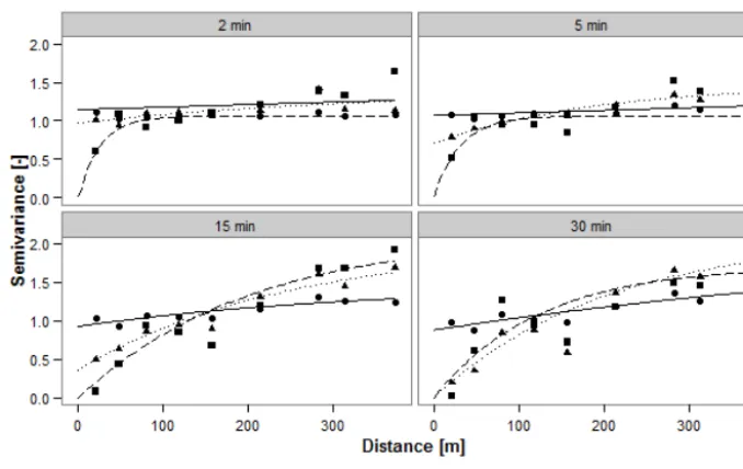
4.1 Calibration of the geostatistical model of rainfall As explained in Sect. 3.4, the geostatistical model of trans-formed rainfall data were calibrated using variograms for three different intensity ranges. This procedure was repeated for temporal averaging intervals of 2, 5, 15, and 30 min.
Ex-ponential models were fitted to empirical variograms. The resulting variograms are presented in Fig. 7.
The variograms illustrate two properties of the collected rainfall measurements: spatial variability of rainfall and mea-surement error. One of the main parameters which charac-terises these properties is the nugget. Theoretically at zero lag distance the variance should be zero. However, most of the variograms exhibit a positive nugget effect (generally presented as nugget-to-sill ratio) at zero lag distance. This nugget effect can be due to two reasons: random measure-ment error and microscale spatial variability of rainfall. Un-fortunately we cannot quantify these causes individually us-ing the variograms. But there is a consistent pattern of nugget against both rainfall intensity class and temporal averaging interval which helps to interpret the variograms.
exam-Figure 7.Calculated variograms for each intensity class within each temporal averaging interval.
ple, for rainfall intensity class 5.0–10.0 mm h−1the nugget-to-sill ratio decreases from almost one to zero as the temporal averaging interval increases from 2 to 30 min. Overall these observations show that the combined effect of random mea-surement error and microscale special variability of rainfall characterised by nugget-to-sill ratio decreases with increas-ing (a) rainfall intensity class and (b) averagincreas-ing interval.
Regarding the behaviour of the nugget-to-sill ratio against averaging interval, it is expected that with the averaging in-terval the (microscale) spatial correlation of rainfall would increase, which partly explains the observed pattern. The increase in spatial correlation of rainfall intensity with in-creasing temporal averaging interval agrees with other simi-lar studies (e.g. Ciach and Krajewski, 2006; Fiener and Auer-swald, 2009; Krajewski et al., 2003; Peleg et al., 2013; Vil-larini et al., 2008). For example, Krajewski et al. (2003) ob-served in their study on analysis of spatial correlation struc-ture of small-scale rainfall in central Oklahoma a similar be-haviour using correlogram functions for different temporal averaging intervals. But commenting on the decreasing trend of the nugget-to-sill ratio against intensity class, it cannot be attributed to improvement in microscale spatial correlation as it is neither natural nor proven. In fact, in Fig. 7 the be-haviour of spatial correlation against rainfall intensity class does not show a distinctive trend except at the origin, i.e. the nugget effect. The absence of any consistent trend of spatial variability against intensity class was also observed in Ciach and Krajewski (2006). Meanwhile this decreasing trend of nugget-to-sill ratio against rainfall intensity corresponds well with measurement errors of tipping bucket type rain gauges caused by its sampling mechanism (hereafter referred to as TB error). This is due to the rain gauges’ inability to cap-ture small temporal variability of the rainfall time series. The
behaviour of TB error against rainfall intensity as seen from Fig. 7 complements results from previous studies (Habib et al., 2001; Villarini et al., 2008). These studies also show that the TB error decreases with temporal averaging interval. Habib et al. (2001) found similar behaviour of TB error with increasing intensity (0–100 mm h−1) and also with increas-ing averagincreas-ing interval (1, 5, and 15 min). Although the bucket size used in their study (0.254 mm) is slightly different from our rain gauge bucket size of 0.2 mm, the characteristic of the TB error against rainfall intensity for different averaging in-terval is consistent in both cases. In summary, the behaviour of nugget-to-sill ratio of the variograms against temporal av-eraging interval can be explained by the combined effect of microscale spatial variability of rainfall and TB error, while the behaviour of nugget-to-sill ratio against intensity range can mainly be attributed to the latter.
In addition to the nugget-to-sill ratio, another parameter that characterises the variograms is the range, i.e. the dis-tance up to which there is spatial correlation. At lower tempo-ral averaging intervals (≤5 min) the variograms for all rain-fall intensity classes reach the variogram range very quickly (< 100 m). But at averaging intervals≥15 min, the range has not been reached even at a maximum separation distance, showing the improvement in spatial correlation. High spatial variability of rainfall at shorter temporal averaging interval (≤5 min) is an important observation in the context of ur-ban drainage runoff modelling, as the time step used in such models is generally around 2 min for small catchments.
[image:9.612.129.468.65.279.2]16 months – Jaffrain and Berne, 2012). These time peri-ods are reflection of the practical and funding issues to maintain such dense networks operating accurately for ex-tended periods. The characteristics of our data are compara-ble with Ciach and Krajewski (2006) and Fiener and Auer-swald (2009) as these studies also used rainfall data from warm months to investigate the spatial correlation structure. Despite the fact that the data cover only 10 months all de-rived variogram models are stable and reliable. Webster and Oliver (2007) suggested around 100 samples to reliably es-timate a variogram model. Even in the case of 30 min tem-poral averaging interval and > 10 mm h−1(where we had the fewest number of observations) we had a total of 196 spa-tial lags to calculate the variogram. Furthermore, we demon-strated that all derived variogram models are stable and reli-able by examining sub-sets of the data. We randomly selected 80 % of the data from each intensity class and reproduced the variograms to compare them with the variograms presented in Fig. 7. We had to limit the subclass percentage to 80 % to give enough time instants to reproduce variograms for all subclasses. We repeated this procedure a few times. Compar-ing these variograms with Fig. 7 shows that these variograms are very similar. One set of the variograms computed from 80 % of the data are presented in the Supplement. This anal-ysis supports our claim that the variograms shown in Fig. 7 are stable and an adequate representation of the rainfall spa-tial variation for each intensity class and temporal averaging interval.
One of the assumptions we made during the pooling pro-cedure is that the spatial variability is reasonably consistent within a pooled intensity class. We acknowledge that with narrower intervals the assumption of consistency in spatial variability would be more realistic. But with the available data we had to find a compromise with the number of time instants. We believe that using three intensity subclasses is a reasonable compromise. Further we also introduced step 2 (Sect. 3.2) which standardises the rainfall for each time in-stant within a subset. Although variograms are derived only for the whole subset, step 2 (before geostatistical upscal-ing) and step 9 (after geostatistical upscalupscal-ing) ensure that the probabilistic model is adjusted for each time instant sepa-rately. Effectively, we assume the same correlogram for time instants of the same subclass, not the same variogram. Al-though this does not justify the assumption of similar spa-tial correlation structure within the pooled classes, it at least relaxes the assumption of the same variogram within sub-classes. To compare the behaviour of variogram models for a narrower intensity interval, we produced variograms for nar-rower intensity classes ranging from 0 to 14 mm h−1for the 5 min averaging interval. The highest intensity class is lim-ited to ≥12 to < 14 mm h−1 as for further narrower ranges (i.e ≥14 to < 16 mm h−1 and so on) there are not enough sample points to produce a meaningful variogram. Narrower intensity classes means that the assumption of similar spatial variability within a pooled subset is more realistic.
Compar-Figure 8.Calculated variograms for a narrower range of intensity at 5 min averaging interval.
ing Figs. 7 and 8, we conclude that the variograms shown in Fig. 7 are accurate representations of the average spatial variability conditions for corresponding intensity classes. 4.2 Geostatistical upscaling of rainfall data
Having calculated all variograms, the next step is to apply spatial stochastic simulation for the time instants of interest followed by steps 6 to 9 in Fig. 4 to calculate the AARI to-gether with associated uncertainty. This procedure was car-ried out for all events presented in Table 1. The following sections present and discuss the predicted AARI and associ-ated uncertainty levels derived from step 9.
4.2.1 Prediction error vs. AARI
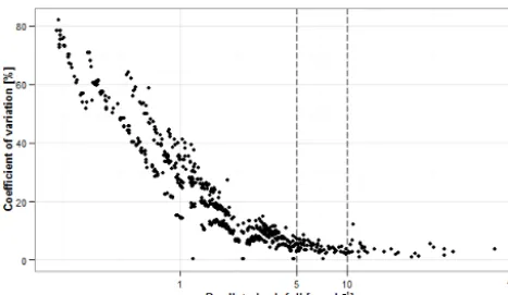
The scatter plot in Fig. 9 shows the coefficient of variation of the prediction error (CV; see Eq. 6) plotted against predicted AARI at 5 min averaging interval for all time instants of all events presented in Table 1:
CV=AARI prediction error standard deviation
[image:10.612.307.549.67.207.2]Figure 9.AARI prediction error CV (%) values against predicted AARI for averaging interval of 5 min.
causing higher uncertainty in the prediction of AARI. At in-tensity class 0–5 mm h−1the nugget-to-sill ratio was almost one (nugget variogram) and as a result the derived CV values are significantly higher than other two intensity classes. It is interesting to note that, in the range of 1–10 mm h−1, there are few points that are separated from the larger cluster with almost zero CV. It shows a consistent rainfall measurement over the area at these time instants, which results in a very small CV in the predicted AARI.
The above discussion is based on results from 5 min tem-poral averaging interval. The following section discusses the effect of temporal averaging interval on prediction error. Fur-ther, although CV in Fig. 9 gets as high as 80 %, the corre-sponding AARI is less than 1 mm h−1, thus the prediction error has a very less significance in urban hydrology. Hence we also analysed the prediction error associated with rainfall events’ peaks in the last section.
4.2.2 Prediction error vs. temporal averaging interval Having analysed the behaviour of the prediction error CV against predicted AARI, this section presents the effect of temporal averaging interval on the prediction error of AARI. Figure 10 shows the kriging predictions with 95 % predic-tion intervals derived from the predicpredic-tion standard deviapredic-tion for temporal averaging intervals of 2, 5, 15, and 30 min for event 11. Event 11 has average conditions in terms of event duration and peak intensity. Prediction errors of other events against the temporal averaging interval follow the same pat-tern of behaviour.
While short time intervals are of greater interest in urban hydrology, they also lead to large uncertainties. Figure 10 shows the smaller the temporal averaging interval, the larger the prediction interval and the larger the level of uncertainty. This is due to the combined effect of higher spatial variability and larger TB error at lower temporal averaging interval as seen from Fig. 7. When the averaging interval is larger than 15 min the prediction interval width becomes negligible. But temporal scales of interest in urban hydrology of a
similar-sized catchment can be as low as 2 min where there is still considerable uncertainty. The 95 % prediction interval shows around±13 % of error in rainfall intensity corresponding to a prediction of peak rainfall of 47 mm h−1at 2 min averaging interval. While temporal aggregation decreases uncertainty, it obviously leads to a significant reduction of the predicted peaks of AARI. For example, the peak of event 11 gets re-duced to around 20 mm h−1 from around 50 mm h−1 when averaging interval increases from 2 to 30 min. Hence a care-ful trade-off between temporal resolution and accuracy in rainfall prediction is needed to decide the most appropriate time step for averaging point rainfall data for urban hydro-logic applications.
The decreasing trend of uncertainty in the prediction of AARI with increasing temporal averaging interval agrees with a previous study by Villarini et al. (2008). Although the spatial extent of their study is much larger (360 km2), their results also show that the spatial sampling uncertainties tend to decrease with increasing temporal averaging interval due to improvement in measurement accuracy and improved spa-tial correlation.
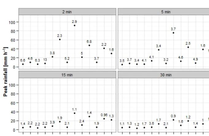
4.2.3 Prediction error vs. peak rainfall intensity In addition to rainfall event durations, rainfall event peaks are also of significant interest in urban hydrology as most of the hydraulic structures in urban drainage systems are de-signed based on peak discharge which is often derived from peak rainfall. Hence it is important to consider the uncer-tainty in prediction of peaks of AARI. Figure 11 presents predicted peaks of AARI for all 13 events presented in Ta-ble 1, together with labels indicating corresponding CV (%) values. The peak intensities range from 6 to 92 mm h−1 at 2 min averaging interval and this range narrows down to 3– 21 mm h−1at averaging interval of 30 min as a result of tem-poral aggregation. As expected, temtem-poral aggregation from 2 to 30 min also results in the reduction of CV. The highest CV at 2 min averaging intervals is 13 % for event 4 and re-duces to 1.7 % at 30 min averaging interval. But it can also be noted that events 5, 6, 8, and 11 show their highest CV at 5 min averaging interval and not at 2 min averaging interval. Tracking back these events, they indeed show more spatial variation over 5 min period compared to 2 min period around the peak.
Figure 10.Predictions of AARI (indicated by points) together with 95 % prediction intervals (indicated by grey ribbon) for rainfall event 11 for different averaging intervals.
Figure 11.Predictions of event peaks of AARI (indicated by points) together with labels indicating corresponding CV (%) values.
higher (> 10 mm h−1) rainfall intensity respectively. Even though these values are significantly less than what we ob-served from Fig. 9 when the rainfall intensity is less than 1 mm h−1, they are still high considering the required ac-curacy defined in standard guidelines of urban hydrological modelling practice. For example, the current urban drainage verification guideline (WaPUG, 2012) in the UK defines a maximum allowable deviation of 25 to−15 % in peak runoff demanding more accurate prediction of rainfall which is the
[image:12.612.128.469.337.559.2]5 Conclusions
Geostatistical methods have been used to analyse the spatial correlation structure of rainfall at various spatial scales, but its application to estimate the level of uncertainty in rainfall upscaling has not been fully explored mainly due to its in-herent complexity and demanding data requirements. In this study we presented a method to overcome these challenges and predict AARI together with associated uncertainty using geostatistical upscaling. We used a spatial stochastic simula-tion approach to address the combinasimula-tion of change of sup-port (from point to catchment) and non-normality of rain-fall observations for prediction of AARI and the associated uncertainty. We addressed the issue of scarcity in measure-ment points by using repetitive rainfall measuremeasure-ments (pool-ing) to increase the number of spatial samples used for var-iogram estimation. The methods were illustrated with rain-fall data collected from a cluster of eight paired rain gauges in a 400 m×200 m urban catchment in Bradford, UK. The spatial lag ranges from 21 to 399 m. As far we are aware these are the smallest lag ranges in which spatial variability in rainfall is examined in an urban area using point rainfall measurements. We defined intensity classes and derived dif-ferent geostatistical models (variograms) for each intensity class separately. We also used different temporal averaging intervals, ranging from 2 to 30 min, which are of interest in urban hydrology. To the best of our knowledge this is the first such attempt to assign geostatistical models for a com-bination of intensity class and temporal averaging interval. Finally, we quantified the level of uncertainty in the predic-tion of AARI for these different combinapredic-tions of temporal averaging intervals and rainfall intensity ranges.
A summary of the significant findings is listed below: – Several studies (e.g. Berne et al., 2004; Gebremichael
and Krajewski, 2004; Krajewski et al., 2003) used a single geostatistical model in the form of vari-ogram/correlogram for the entire range of rainfall in-tensity. The current study shows that for small time and space scales the use of a single geostatistical model based on a single variogram is not appropriate and a dis-tinction between rainfall intensity classes and length of temporal averaging intervals should be made.
– The level of uncertainty in the prediction of AARI us-ing point measurement data essentially comes from two sources: spatial variability of the rainfall and measure-ment error. The significance and characteristics of the measurement error observed here mainly corresponds to sampling related error of tipping bucket type rain gauges (TB error) and may vary for other types of rain gauges.
– TB error decreases with increasing rainfall intensity. As a result of that, the prediction error decreases with in-creasing AARI. At 5 min averaging interval the CV
val-ues are as high as 80 % when the AARI is smaller than 1 mm h−1and they get reduced to less than 10 % when AARI is larger than 10 mm h−1.
– At smaller temporal averaging intervals, the effect of both spatial variability and TB error is high, resulting in higher uncertainty levels in the prediction of AARI. With increasing temporal averaging interval the uncer-tainty becomes smaller as the spatial correlation in-creases and the TB error reduces. At 2 min temporal averaging interval the average CV in the prediction of peak AARI is 6.6 % and the maximum CV is 13 % and they are reduced to 1.5 and 3.6 % respectively at 30 min averaging interval.
– TB error at averaging intervals of less than 5 min, espe-cially at low-intensity rainfall measurements, is as sig-nificant as spatial variability. Hence proper attention to TB error should be given in any application of these measurements, especially in urban hydrology, where av-eraging intervals are often as small as 2 min.
Although the spatial stochastic simulation method used in this study needs more computational power (a summary on computation power is presented in the Supplement) than block kriging, it is a robust approach and allows data trans-formation during spatial interpolation and aggregation. Such data transformation is important because rainfall data are not normally distributed for small temporal averaging inter-vals. The pooling procedure used in this study helps pro-vide a solution to meet the data requirements for geosta-tistical methods as it extends the available information for variogram estimation. Commenting on the minimum num-ber of measurement points needed to employ this method is difficult, because like any other geostatistical interpolation method, the efficiency of this method also heavily depends on reliable estimation of the geostatistical model (variogram). Hence, it basically comes down to the question of whether or not a given measurement network can produce a meaning-ful variogram. As mentioned, Webster and Oliver (2007) ad-vised that around 100 measurement points are needed to ade-quately estimate a geostatistical model. But there is no single universal rule to define the minimum number of bins and the number of samples for each bin to produce a reliable vari-ogram. Further, since pooling sample variograms of repeated measurements would produce a multiplication of spatial lags, the size of the available data set would also play a role in de-ciding the minimum number of measurement points.
gauge data similar to the ones used in this study are crucial for similar studies focused on small urban catchments.
Results from this study can be used for uncertainty anal-yses of hydrologic and hydrodynamic modelling of similar-sized urban catchments in similar climates as it provides in-formation on uncertainty associated with rainfall estimation which is arguably the most important input in these models. This information will help to differentiate input uncertainty from total uncertainty thereby helping to understand other sources of uncertainty due to model parameter and model structure. This estimate of the relative importance of uncer-tainty sources can help to avoid false calibration and force fitting of model parameters (Vrugt et al., 2008). This study can also help to judge optimal temporal averaging interval for rainfall estimation of hydrologic and hydrodynamic mod-elling especially for small urban catchments.
6 Data availability
The rainfall intensity data used in this study are freely avail-able at https://doi.org/10.5281/zenodo.291372.
The Supplement related to this article is available online at doi:10.5194/hess-21-1077-2017-supplement.
Competing interests. The authors declare that they have no conflict of interest.
Acknowledgements. This research was done as part of the Marie Curie ITN – Quantifying Uncertainty in Integrated Catchment Studies (QUICS) project. This project has received funding from the European Union’s Seventh Framework Programme for research, technological development and demonstration under grant agreement no. 607000.
Edited by: P. Molnar
Reviewed by: two anonymous referees
References
Berne, A., Delrieu, G., Creutin, J. D., and Obled, C.: Tem-poral and spatial resolution of rainfall measurements re-quired for urban hydrology, J. Hydrol., 299, 166–179, doi:10.1016/j.jhydrol.2004.08.002, 2004.
Bogner, K., Pappenberger, F., and Cloke, H. L.: Technical Note: The normal quantile transformation and its application in a flood forecasting system, Hydrol. Earth Syst. Sci., 16, 1085–1094, doi:10.5194/hess-16-1085-2012, 2012.
Chow, V. T.: Handbook of Applied Hydrology. A compendium of water-resources technology, McGraw-Hill, New York, 1964.
Ciach, G. J. and Krajewski, W. F.: Analysis and model-ing of spatial correlation structure in small-scale rainfall in Central Oklahoma, Adv. Water Resour., 29, 1450–1463, doi:10.1016/j.advwatres.2005.11.003, 2006.
Dirks, K. N., Hay, J. E., Stow, C. D., and Harris, D.: High-resolution studies of rainfall on Norfolk Island Part II: Interpolation of rainfall data, J. Hydrol., 208, 187–193, doi:10.1016/S0022-1694(98)00155-3, 1998.
Emmanuel, I., Andrieu, H., Leblois, E., and Flahaut, B.: Temporal and spatial variability of rainfall at the ur-ban hydrological scale, J. Hydrol., 430–431, 162–172, doi:10.1016/j.jhydrol.2012.02.013, 2012.
Fankhauser, R.: Influence of systematic errors from tipping bucket rain gauges on recorded rainfall data, Water Sci. Technol., 37, 121–129, doi:10.1016/S0273-1223(98)00324-2, 1998.
Fiener, P. and Auerswald, K.: Spatial variability of rainfall on a sub-kilometre scale, Earth Surf. Processes, 34, 848–859, doi:10.1002/esp.1779, 2009.
Gebremichael, M. and Krajewski, W. F.: Assessment of the statistical characterization of small-scale rainfall variabil-ity from radar: Analysis of TRMM ground validation datasets, J. Appl. Meteorol., 43, 1180–1199, doi:10.1175/1520-0450(2004)043<1180:AOTSCO>2.0.CO;2, 2004.
Gires, A., Onof, C., Maksimovic, C., Schertzer, D., Tchiguirinskaia, I., and Simoes, N.: Quantifying the impact of small scale un-measured rainfall variability on urban runoff through multifrac-tal downscaling: A case study, J. Hydrol., 442–443, 117–128, doi:10.1016/j.jhydrol.2012.04.005, 2012.
Gires, A., Tchiguirinskaia, I., Schertzer, D., Schellart, A., Berne, A., and Lovejoy, S.: Influence of small scale rainfall variability on standard comparison tools between radar and rain gauge data, At-mos. Res., 138, 125–138, doi:10.1016/j.atmosres.2013.11.008, 2014.
Glasbey, C. A. and Nevison, I. M.: Modelling Longitudinal and Spa-tially Correlated Data, edited by: Gregoire, T. G., Brillinger, D. R., Diggle, P. J., Russek-Cohen, E., Warren, W. G., and Wolfin-ger, R. D., SprinWolfin-ger, New York, 233–242, 1997.
Goovaerts, P.: Estimation or simulation of soil properties? An opti-mization problem with conflicting criteria, Geoderma, 97, 165– 186, doi:10.1016/S0016-7061(00)00037-9, 2000.
Habib, E., Krajewski, W. F., and Kruger, A.: Sampling Errors of Tipping-Bucket Rain Gauge Measurements, J. Hydrol. Eng., 6, 159–166, doi:10.1061/(ASCE)1084-0699(2001)6:2(159), 2001. Isaaks, E. H. and Srivastava, R. M.: An Introduction to Applied
Geostatistics, Oxford University Press, New York, USA, 1989. Jaffrain, J. and Berne, A.: Quantification of the small-scale
spa-tial structure of the raindrop size distribution from a net-work of disdrometers, J. Appl. Meteorol. Clim., 51, 941–953, doi:10.1175/JAMC-D-11-0136.1, 2012.
Krajewski, W. F., Ciach, G. J., and Habib, E.: An analysis of small-scale rainfall variability in different climatic regimes, Hydrolog. Sci. J., 48, 151–162, doi:10.1623/hysj.48.2.151.44694, 2003. Lloyd, C. D.: Assessing the effect of integrating elevation data into
the estimation of monthly precipitation in Great Britain, J. Hy-drol., 308, 128–150, doi:10.1016/j.jhydrol.2004.10.026, 2005. Ly, S., Charles, C., and Degré, A.: Different methods for spatial
Mair, A. and Fares, A.: Comparison of Rainfall Interpolation Methods in a Mountainous Region of a Tropical Island, J. Hydrol. Eng., 16, 371–383, doi:10.1061/(ASCE)HE.1943-5584.0000330, 2011.
MetOffice UK: MetOffice, UK, available at: http://www.metoffice. gov.uk/, last access: December 2016.
Montanari, A. and Brath, A.: A stochastic approach for assess-ing the uncertainty of rainfall-runoff simulations, Water Resour. Res., 40, 1–11, doi:10.1029/2003WR002540, 2004.
Nalder, I. A. and Wein, R. W.: Spatial interpolation of climatic Normals: test of a new method in the Canadian boreal for-est, Agr. Forest Meteorol., 92, 211–225, doi:10.1016/S0168-1923(98)00102-6, 1998.
Ochoa-Rodriguez, S., Wang, L. P., Gires, A., Pina, R. D., Reinoso-Rondinel, R., Bruni, G., Ichiba, A., Gaitan, S., Cristiano, E., van Assel, J., Kroll, S., Murlà-Tuyls, D., Tisserand, B., Schertzer, D., Tchiguirinskaia, I., Onof, C., Willems, P., and ten Veldhuis, M. C.: Impact of spatial and temporal resolu-tion of rainfall inputs on urban hydrodynamic modelling out-puts: A multi-catchment investigation, J. Hydrol., 531, 389–407, doi:10.1016/j.jhydrol.2015.05.035, 2015.
Pebesma, E. J.: Multivariable geostatistics in S: The gstat package, Comput. Geosci., 30, 683–691, doi:10.1016/j.cageo.2004.03.012, 2004.
Pedersen, L., Jensen, N. E., Christensen, L. E., and Madsen, H.: Quantification of the spatial variability of rainfall based on a dense network of rain gauges, Atmos. Res., 95, 441–454, doi:10.1016/j.atmosres.2009.11.007, 2010.
Peleg, N., Ben-Asher, M., and Morin, E.: Radar subpixel-scale rain-fall variability and uncertainty: lessons learned from observa-tions of a dense rain-gauge network, Hydrol. Earth Syst. Sci., 17, 2195–2208, doi:10.5194/hess-17-2195-2013, 2013. Schuurmans, J. M. and Bierkens, M. F. P.: Effect of spatial
distri-bution of daily rainfall on interior catchment response of a dis-tributed hydrological model, Hydrol. Earth Syst. Sci., 11, 677– 693, doi:10.5194/hess-11-677-2007, 2007.
Seo, B.-C. and Krajewski, W. F.: Scale Dependence of Radar Rain-fall Uncertainty: Initial Evaluation of NEXRAD’s New Super-Resolution Data for Hydrologic Applications, J. Hydrometeorol., 11, 1191–1198, doi:10.1175/2010JHM1265.1, 2010.
Sevruk, B. and Hamon, W. R.: International comparison of national precipitation gauges with a reference pit gauge, Instruments and Observing Methods, Report No. 17, WMO/TD-No. 38, World Meteorological Organization, Geneva, Switzerland, 1984. Tabios III, G. Q. and Salas, J. D.: A comparative analysis of
tech-niques for spatial interpolation of precipitation, J. Am. Water Re-sour. As., 21, 365–380, 1985.
Todini, E.: A model conditional processor to assess predictive un-certainty in flood forecasting, Int. J. River Basin Manag., 6, 123– 137, doi:10.1080/15715124.2008.9635342, 2008.
Viessman Jr., W. and Lewis, G. L.: Introduction to hydrology, in: Introduction to hydrology, Harper Collins, p. 311, 1995. Villarini, G., Mandapaka, P. V., Krajewski, W. F., and Moore, R. J.:
Rainfall and sampling uncertainties: A rain gauge perspective, J. Geophys. Res.-Atmos., 113, 1–12, doi:10.1029/2007JD009214, 2008.
Van der Waerden, B. L.: Order tests for two-sample problem and their power, Indag. Math., 14, 453–458, 1952.
Vrugt, J. A., ter Braak, C. J. F., Clark, M. P., Hyman, J. M., and Robinson, B. A.: Treatment of input uncertainty in hy-drologic modeling: Doing hydrology backward with Markov chain Monte Carlo simulation, Water Resour. Res., 44, W00B09, doi:10.1029/2007WR006720, 2008.
WaPUG: Code of Practice For The Hydraulic Modelling of Sewer Systems, Wastewater Planning Users Group, UK, 2002. Webster, R. and Oliver, M. A.: Geostatistics for environmental
sci-entists, Second Edn., John Wiley & Sons, Ltd, West Sussex, Eng-land, 2007.