www.hydrol-earth-syst-sci.net/20/4129/2016/ doi:10.5194/hess-20-4129-2016
© Author(s) 2016. CC Attribution 3.0 License.
Relative impacts of land use and climate change on summer
precipitation in the Netherlands
Emma Daniels1, Geert Lenderink2, Ronald Hutjes1, and Albert Holtslag1
1Wageningen University, Droevendaalsesteeg 3, 6708 PB Wageningen, the Netherlands 2KNMI, Utrechtseweg 297, 3731 GA De Bilt, the Netherlands
Correspondence to:Emma Daniels (emmadamme@gmail.com)
Received: 25 March 2016 – Published in Hydrol. Earth Syst. Sci. Discuss.: 6 April 2016 Revised: 14 September 2016 – Accepted: 15 September 2016 – Published: 11 October 2016
Abstract.The effects of historic and future land use on pre-cipitation in the Netherlands are investigated on 18 summer days with similar meteorological conditions. The days are selected with a circulation type classification and a cluster-ing procedure to obtain a homogenous set of days that is ex-pected to favor land impacts. Changes in precipitation are investigated in relation to the present-day climate and land use, and from the perspective of future climate and land use. To that end, the weather research and forecasting (WRF) model is used with land use maps for 1900, 2000, and 2040. In addition, a temperature perturbation of +1◦C assuming constant relative humidity is imposed as a surrogate climate change scenario. Decreases in precipitation of, respectively, 3–5 and 2–5 % are simulated following conversion of historic to present, and present to future, land use. The temperature perturbation under present land use conditions increases cipitation amounts by on average 7–8 % and amplifies pre-cipitation intensity. However, when also considering future land use, the increase is reduced to 2–6 % on average, and no intensification of extreme precipitation is simulated. In all, the simulated effects of land use changes on precipitation in summer are smaller than the effects of climate change, but are not negligible.
1 Introduction
Humans can exert influence on precipitation through modifi-cations in land use (Mahmood et al., 2014; Kalnay and Cai, 2003) next to other anthropogenic forcings such as climate change (Zhang et al., 2007). Currently, land conversion takes place at a rapid pace, and this will likely continue in the
fu-ture (Mahmood et al., 2010; Angel et al., 2011). Therefore, this type of human influence on the climate system will con-tinue, and will probably become more significant in the com-ing decades (Pielke et al., 2007; Mahmood et al., 2010).
In the Netherlands, the most important land cover changes in the last century were the conversion of large heather areas into agricultural land or grassland, and expansion of urban areas (Feranec et al., 2010; Verburg et al., 2004). In addi-tion, almost 1650 km2 of land was reclaimed from the sea in the former Zuiderzee, now called Lake Yssel (Hoeksema, 2007). Urban areas have increased from about 2 % in 1900 to 13 % in 2000, and are projected to further increase to 24 % in 2040 (Dekkers et al., 2012). Precipitation in the Netherlands has increased by about 25 % over the last century, especially along the West coast (Buishand et al., 2013). The increase in sea surface temperatures and changes in circulation seem to be the major causes of this increase (Attema et al., 2014; van Haren et al., 2013). In addition, there is some evidence that urbanization plays a role (Daniels et al., 2015b).
were conceptual, rather than realistic, and only focused on changes in urban extent, ignoring the expansion of agricul-tural areas for example.
The present study aims to improve on both aspects, by (1) sampling a larger set of meteorological cases, and (2) evaluating the effects of more realistic land cover changes. Our main interest is the precipitation response to the al-tered land surface and the physical processes underlying this response. We investigate this response in the summer sea-son. The summer months typically have a larger shower ac-tivity, connected to unstable conditions. This relatively in-tense type of precipitation, arising from (deep) cumulus con-vection, is expected to be most influenced by land surface changes (Pielke et al., 2007; Cotton and Pielke, 2007) and is typically expected to increase under climate change (Fischer et al., 2014). Also, the largest impact of urban areas on pre-cipitation along the Dutch West coast was found in summer (Daniels et al., 2015b).
The current study also aims to put the effects of historic and future land use changes on precipitation in the perspec-tive of climate change. This will be done by imposing an in-crease in overall temperatures as a surrogate climate change scenario (Schar et al., 1996). On a global scale, climate change is expected to increase both mean and extreme pre-cipitation in response to an intensification of the hydrological cycle (Huntington, 2006; Wu et al., 2013). Here, the precip-itation response to land use changes in the Netherlands, and climate change, is investigated for multiple summer days. The selection procedure for the investigated events and the model setup will be described in the next section, followed by the results, discussion, and conclusions.
2 Data and methods 2.1 Case selection
Selection of days to use as case studies is conducted with the help of a circulation type classification, similar to Daniels et al. (2015a). We make use of the nine-type Jenkinson– Collison types (JCT) classification scheme. This method was developed by Jenkinson and Collison (1977) and is intended to provide an objective scheme that acceptably reproduces the subjective Lamb weather types (Jones et al., 1993; Lamb, 1950). The classification has eight weather types (WTs) rep-resentative of the prevailing wind direction (W, NW, N, NE, E, SE, S, and SW, where W=1, etc.) and one that is treated as unclassified (WT9). Computation of the WTs is done us-ing 12:00 UTC MSLP data from ERA-Interim (Dee et al., 2011) at 16 points in the area 47.25 to 57.75◦N and 3 to 12.75◦E (Fig. 1) with the “cost733class” software (Philipp et al., 2010, 2014).
Previous work has shown that the downwind effects of ur-ban areas on precipitation in the Netherlands are largest un-der WT9 (Daniels et al., 2015b). Unun-der the light,
unclassi-fiable, flow that occurs in this weather type, the atmosphere seems to be most susceptible to the land surface. All summer (JJA) days in the period 2000–2010 are classified with the JCT scheme, but only days with WT9 and more than 1 mm of precipitation at one station or more are used for further se-lection. The remaining 215 days are grouped using a statis-tically objectivek-means clustering procedure (Hartigan and Wong, 1979) in R (Core Team, 2013). Thek-means cluster-ing partitionsn observations intokclusters, in which each observation belongs to the cluster with the nearest mean in a principle component space. Clustering is done to obtain a homogenous set of days with similar meteorological condi-tions. The similarity of the cases should result in comparable results and enable generalization of conclusions.
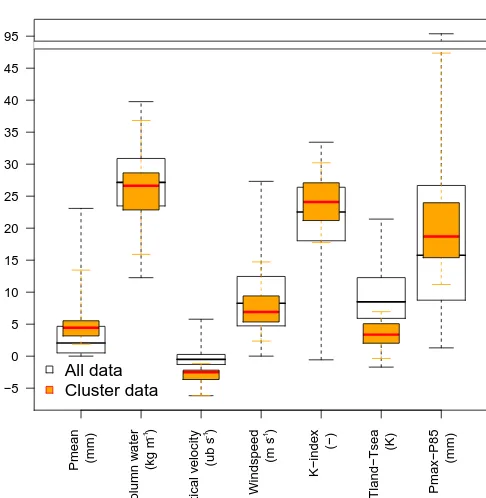
Seven parameters are used in the clustering procedure: (1) mean precipitation; (2) total column water; (3) vertical velocity at 700 hPa; (4) horizontal wind speed at 700 hPa; (5) K-index; (6) land–sea temperature difference; and (7) a measure of the distribution and “patchiness” of precipi-tation, computed as the difference between maximum pre-cipitation and the 85th percentile. Parameters 2, 3, 4, and 5 are derived from 12:00 UTC ERA-Interim data averaged over the center of the Netherlands (4.75 to 5.75◦E and 51.75 to 52.25◦N, Fig. 1). Parameter 6 is derived from ERA-Interim data as the difference between the 2 m temperature over this land area and sea surface temperature (SST) averaged over a nearby ocean area of similar size (3–4◦E and 52.25– 52.75◦N, Fig. 1). Parameter 1 and 7 are computed over the whole of the Netherlands using daily precipitation data col-lected at 08:00 UTC from about 320 stations. TheK-index (George, 1960) is a linear combination of temperature (T) and dewpoint (Td) at various levels (T850−T500+Td850
−(T700−Td700)) and is a measure of the convection used to forecast air mass thunderstorms. The parameter values are normalized and scaled by subtracting the mean and dividing by the standard deviation, before being used in the clustering algorithm.
Figure 1.Map of part of Europe showing the 16 (red) points used in the circulation type classification, the WRF model domain (black), and the land (green) and sea (blue) area used for averaging in the selection procedure.
Pmean (mm)
Column w
ater
(kg m )
V
er
tical v
elocity (ub s )
Windspeed
(m s )
K−inde
x
(−)
Tland−Tsea
(K)
Pmax−P85
(mm)
−5 0 5 10 15 20 25 30 35 40 45 95
All data Cluster data
–1 –1 –1
Figure 2.Boxplots of the seven parameters used in the procedure to select days to simulate with the WRF model. Boxes of the days included in the selected cluster are given in orange and boxes of all summer days classified as WT 9 in the period 2000–2010 are given in white.
2009). This could interfere with our land use experiments and is therefore not sought. Finally, the selected cluster has quite
patchy precipitation, indicative of convective conditions as desired. The selected cluster consists of 19 days (see Fig. 6 for the dates), of which 18 will be averaged on an hourly ba-sis for many of the analyses presented in the results section.
2.2 Model setup
We use the non-hydrostatic Advanced Research WRF model (ARW, version 3.4.1) (Skamarock et al., 2008) on a single domain of 1000×1000 km (see Fig. 1). The model has a hor-izontal grid spacing of 2.5 km and the vertical grid contains 40 sigma levels. Atmospheric and surface boundary condi-tions are obtained from ERA-Interim every 6 h. Model output is stored and analyzed on an hourly basis. The model is run for 48 h, including 12 h of spin-up from 12:00 to 00:00 UTC the previous day, 24 h of simulation on the chosen day, and 12 additional hours to be able to compare it to both radar data (00:00–00:00 UTC) and station data (08:00–08:00 UTC).
Following earlier studies with WRF in the Netherlands (e.g., Steeneveld et al., 2011; Daniels et al., 2015a; Theeuwes et al., 2013), we selected the following schemes to represent subgrid processes: the YSU PBL scheme (Hong et al., 2006), the WRF Single-Moment 6-Class Microphysics Scheme (WSM6) (Hong and Lim, 2006), the RRTMG schemes for both longwave and shortwave radiation (Iacono et al., 2008), the Grell 3-D cumulus parameterization scheme (Grell, 1993; Grell and Devenyi, 2002), and the Unified Noah Land Surface Model (Tewari et al., 2004) with the Urban Canopy Model (UCM). The UCM is a single-layer model that has a simplified urban geometry. Included in the UCM are shad-owing from buildings, reflection of shortwave and longwave radiation, the wind profile in the canopy layer, and multi-layer heat transfer equations for roof, wall, and road surfaces (Kusaka et al., 2001; Kusaka and Kimura, 2004).
[image:3.612.46.289.356.605.2]differentia-1900 2000 2040
Urban and built−up land Dryland cropland and pasture Cropland/woodland mosaic
Grassland
Deciduous Broadleaf forest Evergreen Needleleaf forest
Water bodies Herbaceous wetland Barren or Sparsely vegetated
[image:4.612.120.478.64.228.2]Herbaceous tundra
Figure 3.Dutch land use maps for 1900, 2000, and 2040 based on HGN1900, LGN4, and GE2040, respectively.
Table 1.USGS land use category descriptions and parameter settings used in WRF, with the national land use map (HGN, LGN, and GE2040) classes that are reclassified as such.
USGS land Land use z0 Albedo Green vegetation Leaf area Emissivity HGN/LGN class GE2040 class
use category description (m) (–) fraction (%) index (%) description description
1 Urban and built-up land 0.5 0.15 0.1 1 0.88 Buildings and roads Urban area, commercial/
industrial, seaport, building lot, infrastructure
2 Dryland cropland and pasture 0.15 0.17 0.8 5.68 0.985 Crops and bare soil Arable land
6 Cropland/woodland mosaic 0.2 0.16 0.8 4 0.985 Other Recreation – single day,
recreation – stay, perennial crops
7 Grassland 0.12 0.19 0.8 2.9 0.96 Grassland Grassland
11 Deciduous broadleaf forest 0.5 0.16 0.8 3.31 0.93 Deciduous forest Nature – dry
14 Evergreen needle leaf 0.5 0.12 0.7 6.4 0.95 Coniferous forest Nature – dry
16 Water bodies 0.0001 0.08 0 0.01 0.98 Water Water
17 Herbaceous wetland 0.2 0.14 0.6 5.65 0.95 Reed swamps Nature – wet
19 Barren or sparsely vegetated 0.01 0.38 0.01 0.75 0.9 Drifting sands and sandbanks Greenhouse horticulture,
nature – dry
20 Herbaceous tundra 0.1 0.15 0.6 3.35 0.92 Heath land and raised bogs Nature – dry
tion was copied from the LGN map. Therefore, all dry nature in GE2040 was first classified as herbaceous tundra. Next the newly classified herbaceous tundra was reclassified to barren or sparsely vegetated areas, evergreen needle leaf, and de-ciduous broadleaf forest when it overlapped with the areas classified as such in the LGN map.
2.3 Model simulations
Three model simulations, HIS, REF, and FUT, are done with the land use maps of, respectively, 1900, 2000, and 2040 in the Netherlands. These simulations have exactly the same boundary conditions. In 1900 the creation of land in Lake Yssel had not yet taken place. To test the effect of this con-version separately from the changes in land use, an additional simulation with the historic land use map was done, this time with the current land extent (similar to that in REF). All previously non-existent land is assumed to be covered with grassland (the most common land cover class). This simula-tion is referred to as HIS+Ys.
Furthermore, to be able to put the land cover changes in the perspective of climate change, simulations with the present and future land use maps and a temperature perturbation of +1◦C are conducted. These will be referred to as REF+1 and FUT+1. The global surface temperature is predicted to in-crease by at least 1◦C under all concentration pathways by 2050 (IPCC, 2013). The surrogate climate change scenario is applied to the initial land and atmospheric conditions of the simulations, as well as to the driving sea surface temperature following the methodology by Attema et al. (2014), who sug-gest a vertically uniform temperature perturbation is appro-priate at mid-latitudes. The relative humidity is unchanged in these simulations, which implies an absolute surface humid-ity increase of 6–7 %.
[image:4.612.61.536.292.450.2]and because the population density within cities decreased (Marshall, 2007). Within Europe a population density decline rate of 2 % per annum was reached between 1990 and 2000 (Angel et al., 2011). We assume a conservative increase with a decline rate of 1 % for the future. Urban areas are therefore less than doubled in our simulations, consistent with Angel’s projection for Europe and Japan in 2050 with an annual den-sity decline of 1 %.
2.4 Precipitation data
In the Netherlands, measurements of precipitation are avail-able from the national meteorological institute (KNMI). Gauge measurements are available on a daily basis (08:00– 08:00 UTC) at about 320 stations. Gridded observations of precipitation are available at a 2.4 km resolution on an hourly basis from (bias-)corrected radar data (Overeem et al., 2009). Modeled precipitation amounts are best compared with radar data, because of the similarity in resolution and spatial ex-tent. Unfortunately for 4 of the 19 selected cases there are no radar data available, so some averages shown in the results sections consist of fewer cases.
3 Results
The focus of this paper is on the sensitivity of precipitation to changes in land surface conditions in historical and future perspectives. The precipitation response to the perturbations in the experiments will be described in the next section. To clarify these responses, the section after that focusses on the (differences in) atmospheric conditions and processes lead-ing to the formation of precipitation.
In general, the WRF model overestimates precipitation amounts compared to both station and radar data (Fig. 4). The days marked with red markers only have station data, and no radar data are available. There is 1 day where precipitation amounts are grossly overestimated, namely for 30 June 2003. This day is marked with an open dot in the scatterplot. This is the only day in the selection that has easterly winds, and the poor model performance could therefore be related to the chosen position of the domain. This day was excluded from further analysis, so only 18 days are used further on in this paper. The average wind direction on the other days is southwest, like the year-round dominant wind direction in the Netherlands.
The performance of the model in representing spa-tial precipitation patterns is reasonable overall, but shows quite patchy results (Fig. 5). The precipitation pattern of 29 July 2000 for example is well represented by the model. This day is denoted by a triangle in Fig. 4. As an example in which the model does not represent the spatial precipita-tion pattern well, the precipitaprecipita-tion pattern of 22 July 2007 is given. This day is denoted by a square in Fig. 4. Compared to the previous example, this day is more accurately
mod-0 5 10 15
0
5
10
15
20
Observed mean precipitation (mm)
Modelled mean precipitation (mm)
[image:5.612.308.548.64.376.2]Radar Station
Figure 4.Scatterplot of observed and modeled daily mean
precip-itation (mm day−1) by radar (black, 00:00–00:00 UTC) and at
sta-tions (red, 08:00–08:00 UTC) over the Netherlands. The dotted and dashed lines give a linear regression between precipitation modeled and observed by radar, respectively, including and excluding the day indicated with an open dot (30 June 2003). The days with a square (22 July 2007) and triangle (29 July 2000) are illustrated spatially in Fig. 5. The solid 1 : 1 line represents a perfect correlation.
eled in terms of amounts, but the modeled spatial distribu-tion is quite distant from that observed. The average spatial distribution of all 18 cases overestimates the amount of pre-cipitation compared to observed station data by almost 50 %. Nevertheless, the model seems to capture the relatively high precipitation amounts in the center of the country and lower rainfall amounts in the northern parts.
2000−07−29
0 4 8 12 16 20 24 28 32 36 40 44 48 52 56
(mm)
2007−07−22
0 4 8 12 16 20 24 28 32 36 40 44 48 52 56
(mm)
Average
0 1 2 3 4 5 6 7 8 9 10 11 12 13 14
(mm)
2000−07−29
0 4 8 12 16 20 24 28 32 36 40 44 48 52 56
(mm)
2007−07−22
0 4 8 12 16 20 24 28 32 36 40 44 48 52 56
(mm)
Average
0 1 2 3 4 5 6 7 8 9 10 11 12 13 14
[image:6.612.102.498.63.388.2](mm)
Figure 5.Daily mean precipitation (mm day−1) simulated by the model (top) and observed (bottom) on (from left to right) 29 July 2000 and 22 July 2007 (00:00 to 00:00 UTC), and averaged (08:00 to 08:00 UTC) over the 18 selected cases.
HIS HIS+Ys REF REF+1 FUT FUT+1
2000−06−05 2000−07−05 2000−07−29 2001−08−09 2002−08−03 2003−06−30 2003−07−24 2005−08−12 2006−08−09 2006−08−17 2006−08−25 2007−06−24 2007−07−09 2007−07−10 2007−07−22 2008−06−12 2008−06−15 2009−08−25 2010−08−02
Av
e
ra
g
e
Mean
−30 −20 −10 0 10 20 30
Figure 6. Relative precipitation difference (%) in each of the cases for all experiments compared to REF. Here the average is directly calculated over the 18 selected cases and the mean is calculated using the mean spatial differences as given in Fig. 7.
over a different number of cases (14 vs. 18, respectively). Repeating the analysis with the lower number of cases leads to the same results.
3.1 Precipitation response
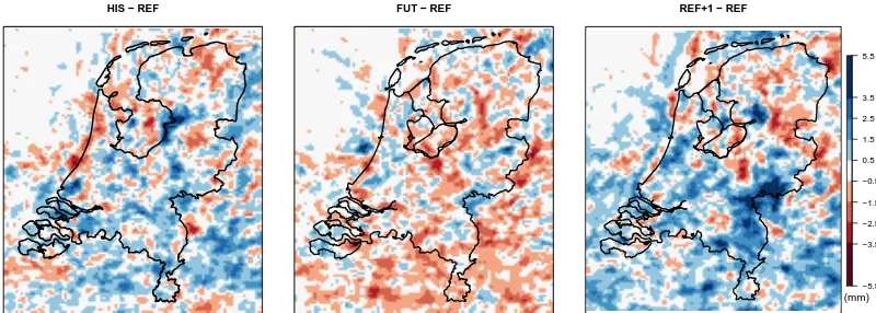
[image:6.612.118.480.434.601.2]be-HIS − REF FUT − REF REF+1 − REF
−5.5 −3.5 −2.5 −1.5 −0.5 0.5 1.5 2.5 3.5 5.5
[image:7.612.100.500.67.210.2](mm)
Figure 7.Spatial precipitation differences (mm day−1) between the HIS, REF+1, and FUT experiments and the reference experiment.
tween the different cases. In Fig. 6 the relative difference of precipitation between the land cover/temperature scenar-ios and REF is given for each of the 19 cases. The average precipitation difference given here is calculated over the 18 cases (excluding the 30 June 2003 case) by averaging the rel-ative change per case. The mean precipitation difference is, on the other hand, directly calculated from the averaged pre-cipitation amount of the 18 cases as given in Fig. 7. Although the strength and sometimes the sign of the response differs between the days in every simulation, a generic picture of a decrease in precipitation appears as a response to changes in land use. From historic to present, and from present to future, land use, the decrease is about 3–5 and 2–5 %, respectively.
One of the averaging methods shows a difference between HIS and HIS+Ys, suggesting that the creation of land in Lake Yssel caused a moderate reduction of precipitation in the last century. The other method gives the same response for both HIS scenarios, suggesting the creation of land in Lake Ys-sel did not influence the total precipitation response. Either way, the model simulates a reduction of precipitation be-tween HIS(+Ys) and REF. Similarly, the difference bebe-tween FUT and REF is negative, so a reduction of precipitation is simulated by the model after incorporation of future land use. On average, the spatial differences between the simula-tions are quite patchy (Fig. 7). All simulasimula-tions show small areas of enhancement as well as areas of reduction in pre-cipitation. The reduction in FUT is seen over large parts of the Netherlands. Urbanization mainly takes place along the West coast, where the reduction of precipitation seems to be moderate. The relatively small reduction might be caused by the downwind enhancement of precipitation by urban ar-eas, though the patchiness in the rest of the country does not seem supportive of this hypothesis. In the HIS simulation, the largest enhancement is located on the eastern side of Lake Yssel. This increase is not visible in the HIS+Ys simulation, so it might be caused by the relatively high SST and evapo-ration over Lake Yssel itself and subsequent higher moisture content of the air when it reaches the coast. The enhancement of precipitation in REF+1 and FUT+1 is most pronounced
along the southeastern border of the country. The relatively large spatial changes shown here average out to the relative changes given before in the order of 2–8 %, which is only 0.1–0.6 mm. So the average changes between the runs are much smaller than the patchy spatial differences seen here.
It is interesting to see whether the precipitation response to the perturbations happens equally throughout the day, or whether it occurs during a specific moment. In the mean daily evolution of precipitation, the differences between HIS(+Ys) and REF are hardly distinguishable (Fig. 8). The differences between FUT and REF manifest themselves in the middle of the day when the intensity of precipitation is lower in FUT. This reduction of precipitation is also seen in FUT+1 and must be caused by land use changes, like the expansion of ur-ban areas. The most pronounced temporal differences are vis-ible in the temperature perturbation experiments: REF+1 and FUT+1. The differences are most evident in the early morn-ing between 02:00 and 08:00 UTC. This difference is not sig-nificant as the divergence is mainly caused by the precipita-tion enhancement on 2000-07-05, the day with the largest response to the temperature perturbations. So the only sys-tematic differences between REF and other simulations are seen in FUT and FUT+1 in the middle of the day.
re-0.0
0.1
0.2
0.3
0.4
0.5
0.6
0.7
Time (UTC)
Mean precipitation (mm)
0 2 4 6 8 10 12 14 16 18 20 22 24
[image:8.612.304.548.65.274.2]HIS_T HIS+Ys REF REF+1 FUT FUT+1 Radar
Figure 8.Diurnal cycle of mean precipitation (mm h−1) over the Netherlands in the different experiments (averaged over 18 cases) and given by radar data (averaged over 14 cases).
1e−06 1e−04 1e−02 1e+00
0
1
02
03
04
05
0
Exceedance probability
Precipitation (mm h )
HIS HIS+Ys REF REF+1 FUT FUT+1 Radar
–1
Figure 9.Distribution of hourly precipitation (mm h−1) for each of the experiments and radar data, averaged over the 14 days that have radar data available.
spectively, to attain the mean and average values in FUT+1, of 6 and 2 %, respectively.
The distribution of precipitation is not well represented by the model, but is consistent among the scenarios (Fig. 9). The extremes of precipitation are very similar in all of the exper-iments, except for REF+1. The REF+1 simulation reveals a considerable increase in precipitation extremes. In the tail of
HIS HIS+Ys REF+1 FUT FUT+1
LH HFX RH
Re
la
ti
v
e
c
h
a
n
g
e
(
%
)
−10
−5
0
5
[image:8.612.45.288.66.286.2]10
Figure 10.Mean relative change (%) over the Netherlands in latent heat flux (LH), sensible heat flux (HFX), and relative humidity (RH) in each of the experiments in comparison to REF.
the distribution the difference with REF is more than 20 %. For more moderate extremes (>15 mm) the difference be-tween REF+1 and REF is about 10 %. Although mean pre-cipitation increases in FUT+1, the distribution remains sim-ilar to REF. Apparently extreme precipitation is in this case influenced more by land use changes than mean precipita-tion. The spatial distribution of the enhanced precipitation is similar to the pattern of mean precipitation; in other words, there is more rain in the same locations. Overall, what can be inferred is that climate change and future land use change have an equal, though opposed, effect on extreme precipita-tion. The atmospheric conditions and relatively little (deep) convection in FUT+1 seem to play a role in the differences between the simulations.
3.2 Surface and atmospheric conditions
[image:8.612.47.289.349.570.2]Table 2.Mean daily (00:00–00:00 UTC) values of latent heat flux (LH), sensible heat (HFX), convective available potential energy (CAPE), precipitation (RAIN), and daytime (06:00–18:00 UTC) values of the percentage of time and area that the planetary boundary layer top is
over the level of free convection (PBL>LFC), likewise for lifting condensation level (PBL>LCL), over the Netherlands for the conducted
experiments.
Variable Unit HIS HIS+Ys REF REF+1 FUT FUT+1
LH W m2 88.6 82.5 81.1 83.7 73.0 75.4
HFX W m2 40.2 38.4 39.4 38.0 43.8 42.6
CAPE J kg−1 330.1 311.4 301.2 360.6 290.1 346.7
PBL>LCL % 54.2 54.0 52.7 52.9 51.0 51.2
PBL>LFC % 45.3 45.0 43.7 44.0 41.7 42.1
RAIN mm day−1 7.5 7.3 7.2 7.7 6.9 7.5
In REF+1 the heat fluxes are not that different from REF. Nevertheless, there is a large precipitation response. The im-posed temperature perturbation with constant relative humid-ity increases the amount of moisture at the time of initial-ization and the amount that enters the model domain at the boundaries, causing precipitation to change, but fluxes to re-main the same. In FUT and FUT+1 a reduction of the latent heat flux is simulated in comparison to REF. Also, in both experiments relative humidity at the surface is lower than in REF. The expansion of urban areas leads to an increase in the sensible heat flux and a decrease in the latent heat flux, since potential evaporation is reduced within urban areas. This de-creases overall moisture availability. The surface responses in FUT and FUT+1 look relatively similar, though the pre-cipitation response relative to REF is of opposite sign in the experiments (Fig. 6).
We now focus on the possibility of triggering convection by considering the atmospheric conditions. Figure 11 shows the median of the diurnal cycle of the planetary boundary layer (PBL), lifting condensation level (LCL), level of free convection (LFC), and convective available potential energy (CAPE) calculated at the lowest model level, of the 18 cases in the REF experiment. We show the median because the mean is influenced more by outliers from individual cases. For REF+1, FUT, and FUT+1, the average difference with regards to REF is given for each of these variables. The dif-ferences are normalized with respect to the mean values in REF, so a relative increase is given at every time. On aver-age, the PBL increases to about 800 m during daytime and reaches the LCL at around 09:00 UTC. In the figure, the LFC remains well above the PBL and LCL. In many in-dividual cases, however, the LFC drops to about 800 m as well, permitting (deep) convection. The LFC reaches its low-est level at 11:00 UTC. This coincides with the time of the highest precipitation intensities in the model (Fig. 8). CAPE increases up to 09:00 UTC, while the LFC decreases and then stabilizes because of the rain and associated temperature and humidity changes. The early onset and intensification of pre-cipitation in the model (Fig. 8) contributes to the small build-up of CAPE and could explain the underestimation of
ex-treme precipitation compared to observations (Fig. 9). Also, there are large spatial variations in these variables. There-fore, we computed the fraction of space and time that the PBL is higher than the LCL and LFC, respectively (Table 2). We consider this a measure of the amount of triggering that occurs.
In REF+1 the temperature is higher, while the PBL is quite similar to REF. During daytime there is little difference be-tween REF and REF+1 regarding the LCL and LFC, and ap-proximately the same amount of triggering (PBL higher than LCL/LFC) occurs (Table 2). At night the LCL and LFC are lower in REF+1 than in REF. CAPE is higher throughout the day in REF+1 than in REF, likely due to the enhanced mois-ture content above the PBL as a result of the imposed climate change scenario. This leads to the simulation of higher pre-cipitation amounts and intensities in REF+1 (Fig. 9). In FUT the large sensible heat flux causes the PBL to grow more dur-ing the day and stay higher durdur-ing the evendur-ing than in REF. The relatively large sensible heat flux also affects and raises the LCL and LFC. In comparison to REF, CAPE decreases in FUT from 08:00 UTC onwards when temperatures go up, and relatively little moisture is available. Consequently, less precipitation is simulated.
0 5
10 15 20
100 200 500 1000 2000 5000
REF
Time (UTC)
Height (m) / CAPE (J kg )
0 5
10 15 20
−0.3 −0.2 −0.1 0.0 0.1 0.2 0.3
REF+1 − REF
Time (UTC)
No
rm
a
liz
e
d
m
e
a
n
d
if
fe
re
n
c
e
0 5 10 15 20
−0.3 −0.2 −0.1 0.0 0.1 0.2 0.3
FUT − REF
Time (UTC)
No
rm
a
liz
e
d
m
e
a
n
d
if
fe
re
n
c
e
PBL LCL LFC CAPE
0 5 10 15 20
−0.3 −0.2 −0.1 0.0 0.1 0.2 0.3
FUT+1 − REF
Time (UTC)
No
rm
a
liz
e
d
m
e
a
n
d
if
fe
re
n
c
e
[image:10.612.127.469.65.405.2]–1
Figure 11.Diurnal cycle of the planetary boundary layer (PBL, solid), lifting condensation level (LCL, dashed), level of free convection
(LFC, dotted) (m), and convective available potential energy (CAPE, dash-dotted) (J kg−1) in the reference experiment and normalized mean
difference of these variables in the experiments with a temperature perturbation and reference land cover (REF+1), future land cover (FUT), and a temperature perturbation and future land cover (FUT+1).
4 Discussion
Although WRF is a widely used atmospheric model, ques-tions regarding the choice of parameterization schemes and the model’s validity for the specific conditions always re-main. The sensitivity to different parameterization schemes was not specifically investigated in this study, while this is known to be important (Gallus and Bresch, 2006; Jankov et al., 2005; Rajeevan et al., 2010; Ruiz et al., 2010; Zeng et al., 2012; ter Maat et al., 2013). The chosen YSU PBL scheme is a first-order nonlocal scheme that is widely used under convective conditions (Hu et al., 2010). Sensitivity to initial conditions was checked for some of the cases by start-ing the runs up to 3 h earlier or later. This had relatively lit-tle effect and WRF seems pretty robust in its predictions, so the sensitivity is small. Previous work (Daniels et al., 2015a) found the largest sensitivity to the initial soil moisture con-ditions. In the Netherlands those conditions are generally at field capacity due to the frequent rain and high groundwater table and can therefore be expected to have limited influence.
The HIS, REF, and FUT experiments were duplicated with-out the convection scheme, but this was found to have little effect on precipitation amounts and is therefore not shown. The utilized and presented model design is consequently only one version of reality, of which many more could be simu-lated.
in summer after expansion of urban land by 40 %. They also found that the area in which precipitation was altered in-creased nearly linearly with the urban land increment.
The utilized procedure to select cases for simulation was intended to obtain a homogeneous set of days with similar meteorological conditions that were thought to favor the land surface impact on precipitation. A large spread among re-sponses to land use and temperature scenarios was found be-tween the cases, however, so the intended comparability was not fully accomplished. This could be a model artefact or a realistic response showing how differently the atmosphere reacts to similar conditions, thus showing natural variabil-ity. Nevertheless, the majority of cases have a similar sign in their response. By averaging the results we find a more representable response then the response of any single case could be. Our estimates could be biased by the selection pro-cedure that selected cases with rather strong convective ac-tivity. Consequently, convection will always be triggered in the selected cases and a potential feedback increasing precip-itation through enhanced triggering was excluded. Examples of this feedback can be found in Findell and Eltahir (2003), Santanello et al. (2011), Taylor et al. (2012), and others. The Netherlands is however not located in a region where strong feedbacks of this type are expected (Seneviratne et al., 2006; The GLACE Team et al., 2004) and the influence of changes in climate, SST, or circulation are likely more important (At-tema et al., 2014; van Haren et al., 2013). If the selection procedure had been more successful in identifying similar events, we could have made a composite event by averaging the initial and boundary conditions, similar to Mahoney et al. (2012). Their procedure sounds promising, because it could reduce simulation time and provide a more representative re-sponse, but the selection of cases to average is apparently not straightforward.
In this study reductions in precipitation from historic to present, as well as from present to future, land use are ob-tained for selected summer cases in the Netherlands. Ob-servations show, however, that precipitation has on aver-age increased by about 25 % in the last century (Buishand et al., 2013). So apparently factors other than land use changes have been dominant. The observed change in pre-cipitation was larger in the winter half-year than the summer half-year nonetheless, and the trend in the summer months (June–August) in the period 1951–2009 was only about 5 % (Daniels et al., 2014). Hence, land surface changes in the last century might have mitigated some of the precipitation increase in summer and hereby have contributed to the rel-atively low increase observed in summer. The same seems to happen in the future in the simulations: combining fu-ture land use with the expected temperafu-ture rise reduces the precipitation increase in the model. This might only hold for summer, however, because historical and theoretical ev-idence suggests that the precipitation response to land use changes is lower in cases with non-convective precipitation (Pielke et al., 2007; Cotton and Pielke, 2007). Studies for
different types of precipitation, taking place in other seasons, are therefore desirable as well.
The climate change scenario used here maintains constant relative humidity in the model. The resulting response in precipitation under current land cover conditions (REF+1) is close to the expected increase in near surface humidity of about 7 % estimated with the Clausius–Clapeyron equa-tion. It is interesting to note that in all simulations, except for REF+1, no differences in extreme precipitation were simu-lated. We note that it is not the changes in mean, but the changes in extreme precipitation that may cause problems for society, with for example landslides or urban flooding (e.g., Feddema et al., 2005; Hibbard et al., 2010; Mahmood et al., 2014). In REF+1 precipitation over 15 mm h−1 increases with 10 % or more. This increase is higher than the average increase in extreme precipitation simulated by global climate models (GCMs), which is about 6 % per degree global warm-ing (Kharin et al., 2007, 2013). Mean precipitation also in-creases more in our simulations (7–8 %) than in GCMs (3 %) (Allen and Ingram, 2002). This can be explained because we investigate hourly data, while GCM data are generally daily, and we only simulate 18 cases, while GCMs generate mean climate simulations. In addition, GCMs generally show a de-crease in the occurrence frequency and an inde-crease in the in-tensity of precipitation. Because we only selected cases in which precipitation occurs, there can be no difference in the occurrence frequency in our simulations. Our estimates are therefore higher than those made by GCMs, but similar to comparable studies (Attema et al., 2014).
5 Conclusions
This paper aims to quantify the precipitation response to his-toric (1900) and future (2040) land use change in the Nether-lands, and to put this response in the perspective of climate change. To achieve this, historic, present, and future land use maps are incorporated into the WRF model. In addi-tion, simulations with a temperature perturbation of+1◦C are done as a surrogate climate change scenario. The inves-tigation is done for 18 summer days with similar character-istics that were selected with a circulation type classification andk-means clustering procedure. On average, precipitation decreases from historic to present land cover by 3–5 %, and decreases by 2–5 % from present to future land cover. Cre-ation of land in Lake Yssel might have caused a decrease in precipitation, but the evidence is not exhaustive. Under the present climate, the simulated land use changes hardly have any influence on extreme precipitation.
the future. Precipitation increases by 7–8 % on average in response to the temperature perturbation in the climate sim-ulations and has a disproportional impact on extremes. Ex-pected land use changes, including the expansion of urban areas, diminish this increase, however. As such an average precipitation increase of 2–6 % is achieved in the simulation that combines future land use with climate change. No in-crease in extreme precipitation is found in the combined fu-ture land use–climate change simulation. Overall, although the precipitation response to land use changes is smaller than the response to climate change, it is not negligible in the sum-mer period in the Netherlands. Our simulations suggest this might be especially true for precipitation extremes.
Author contributions. The authors collectively designed the exper-iments and interpreted the results. Emma Daniels conducted the ex-periments, analyzed the data, and wrote the paper, which all the authors commented on.
Acknowledgements. Emma Daniels and Geert Lenderink acknowl-edge contributions of the Knowlacknowl-edge for Climate program, and Ronald Hutjes and Albert Holtslag acknowledge support by the EU EMBRACE program.
Edited by: B. Schaefli
Reviewed by: two anonymous referees
References
Allen, M. R. and Ingram, W. J.: Constraints on future changes in climate and the hydrologic cycle, Nature, 419, 224–232, doi:10.1038/Nature01092, 2002.
Angel, S., Parent, J., Civco, D. L., Blei, A., and Potere, D.: The dimensions of global urban expansion: Estimates and projec-tions for all countries, 2000–2050, Prog. Plann., 75, 53–107, doi:10.1016/j.progress.2011.04.001, 2011.
Attema, J. J., Loriaux, J. M., and Lenderink, G.: Extreme precipitation response to climate perturbations in an atmo-spheric mesoscale model, Environ. Res. Lett., 9, 12 pp., doi:10.1088/1748-9326/9/1/014003, 2014.
Buishand, T. A., De Martino, G., Spreeuw, J. N., and Brandsma, T.: Homogeneity of precipitation series in the Netherlands and their trends in the past century, Int. J. Climatol., 33, 815–833, doi:10.1002/joc.3471, 2013.
Core Team R.: R: A language and environment for statistical com-puting, R Foundation for Statistical Comcom-puting, Vienna, Austria, 3501 pp., 2013.
Cotton, W. R. and Pielke, R. A.: Human impacts on weather and climate, Cambridge University Press, 2nd edition edn., 332 pp., 2007.
CPB, MNP, and RPB: Welvaart en Leefomgeving, Een scenarios-tudie voor Nederland in 2040, Tech. rep., Den Haag, the Nether-lands, 2006.
Daniels, E. E., Lenderink, G., Hutjes, R. W. A., and Holtslag, A. A. M.: Spatial precipitation patterns and trends in The Netherlands during 1951-2009, Int. J. Climatol., 34, 1773–1784, doi:10.1002/joc.3800, 2014.
Daniels, E. E., Hutjes, R. W. A., Lenderink, G., Ronda, R. J., and Holtslag, A. A. M.: Land surface feedbacks on spring pre-cipitation in the Netherlands, J. Hydrometeorol., 16, 232–243, doi:10.1175/jhm-d-14-0072.1, 2015a.
Daniels, E. E., Lenderink, G., Hutjes, R. W. A., and Holt-slag, A. A. M.: Observed urban effects on precipitation along the Dutch West coast, Int. J. Climatol., 36, 2111–2119, doi:10.1002/joc.4458, 2015b.
Dee, D. P., Uppala, S. M., Simmons, A. J., Berrisford, P., Poli, P., Kobayashi, S., Andrae, U., Balmaseda, M. A., Balsamo, G., Bauer, P., Bechtold, P., Beljaars, A. C. M., van de Berg, L., Bid-lot, J., Bormann, N., Delsol, C., Dragani, R., Fuentes, M., Geer, A. J., Haimberger, L., Healy, S. B., Hersbach, H., Hólm, E. V., Isaksen, L., Kållberg, P., Köhler, M., Matricardi, M., McNally, A. P., Monge Sanz, B. M., Morcrette, J. J., Park, B. K., Peubey, C., de Rosnay, P., Tavolato, C., Thépaut, J. N., and Vitart, F.: The ERA-Interim reanalysis: configuration and performance of the data assimilation system, Q. J. Roy. Meteor. Soc., 137, 553–597, doi:10.1002/qj.828, 2011.
Dekkers, J., Koomen, E., Jacobs Crisioni, C., and Rijken, B.: Scenario-based projections of future land use in the Netherlands: A spatially-explicit knowledge base for the Knowledge for Cli-mate programme, Tech. Rep. SL-11, Department of Spatial Eco-nomics/ Spatial Information Laboratory (SPINlab), Amsterdam, the Netherlands, 2012.
EEA: Corine land cover 2000, European Environment Agency,
available at: http://www.eea.europa.eu/data-and-maps/data/
corine-land-cover-2000-clc2000-seamless-vector-database, 2002.
Feddema, J. J., Oleson, K. W., Bonan, G. B., Mearns, L. O., Buja, L. E., Meehl, G. A., and Washington, W. M.: The importance of land-cover change in simulating future climates, Science, 310, 1674–1678, doi:10.1126/science.1118160, 2005.
Feranec, J., Jaffrain, G., Soukup, T., and Hazeu, G.: Determin-ing changes and flows in European landscapes 1990-2000 using CORINE land cover data, Appl. Geogr., 30, 19–35, doi:10.1016/j.apgeog.2009.07.003, 2010.
Findell, K. L. and Eltahir, E. A. B.: Atmospheric con-trols on soil moisture-boundary layer interactions: Three-dimensional wind effects, J. Geophys. Res.-Atmos., 108, doi:10.1029/2001jd001515, 2003.
Fischer, E. M., Sedlacek, J., Hawkins, E., and Knutti, R.: Mod-els agree on forced response pattern of precipitation and temperature extremes, Geophys. Res. Lett., 41, 8554–8562, doi:10.1002/2014gl062018, 2014.
Gallus, W. A. and Bresch, J. F.: Comparison of impacts of WRF dynamic core, physics package, and initial conditions on warm season rainfall forecasts, Mon. Weather Rev., 134, 2632–2641, doi:10.1175/mwr3198.1, 2006.
George, J. J.: Weather forecasting for aeronautics, New York and London Academic Press, 673 pp., 1960.
Grell, G. and Devenyi, D.: A generalized approach to pa-rameterizing convection combining ensemble and data as-similation techniques, Geophys. Res. Lett., 29, 38-1–38-4, doi:10.1029/2002GL015311, 2002.
Hartigan, J. A. and Wong, M. A.: Algorithm AS 136: A K-Means Clustering Algorithm, J. Roy. Stat. Soc.„ 28, 100–108, doi:10.2307/2346830, 1979.
Hazeu, G., Schuiling, C., Dorland, G., Oldengarm, J., and Gijs-bertse, H.: Landelijk grondgebruiksbestand Nederland versie 6 (LGN6); vervaardiging, nauwkeurigheid en gebruik, tech. rep., Alterra, Wageningen, the Netherlands, 2010.
Hazeu, G. W., Bregt, A. K., de Wit, A. J. W., and Clevers, J. G. P. W.: A Dutch multi-date land use database: Identification of real and methodological changes, Int. J. Appl. Earth Obs., 13, 682–689, doi:10.1016/j.jag.2011.04.004, 2011.
Hibbard, K., Janetos, A., van Vuuren, D. P., Pongratz, J., Rose, S. K., Betts, R., Herold, M., and Feddema, J. J.: Research pri-orities in land use and land-cover change for the Earth system and integrated assessment modelling, Int. J. Climatol., 30, 2118– 2128, doi:10.1002/joc.2150, 2010.
Hoeksema, R. J.: Three stages in the history of land recla-mation in the Netherlands, Irrig. Drain., 56, S113–S126, doi:10.1002/ird.340, 2007.
Hong, S. and Lim, J. J.: The WRF single–moment 6–class micro-physics scheme (WSM6), J. Korean Meteorol. Soc., 42, 129– 151, 2006.
Hong, S.-Y., Noh, Y., and Dudhia, J.: A New Vertical Diffusion Package with an Explicit Treatment of Entrainment Processes, Mon. Weather Rev., 134, 2318–2341, doi:10.1175/mwr3199.1, 2006.
Hu, X.-M., Nielsen Gammon, J. W., and Zhang, F.: Evalu-ation of Three Planetary Boundary Layer Schemes in the WRF Model, J. Appl. Meteorol. Climatol., 49, 1831–1844, doi:10.1175/2010jamc2432.1, 2010.
Huntington, T. G.: Evidence for intensification of the global water cycle: Review and synthesis, J. Hydrol., 319, 83–95, doi:10.1016/j.jhydrol.2005.07.003, 2006.
Iacono, M. J., Delamere, J., Mlawer, E., Shephard, M., Clough, S., and Collins, W.: Radiative forcing by long–lived greenhouse gases: Calculations with the AER radiative transfer models, J. Geophys. Res., 113, 8 pp., doi:10.1029/2008JD009944, 2008. IPCC: Climate Change 2013: The Physical Science Basis.
Con-tribution of Working Group I to the Fifth Assessment Re-port of the Intergovernmental Panel on Climate Change, Tech. rep., Cambridge, UK and New York, NY, USA, doi:10.1017/CBO9781107415324, 2013.
Jankov, I., Gallus, W. A., Segal, M., Shaw, B., and Koch, S. E.: The impact of different WRF model physical parameterizations and their interactions on warm season MCS rainfall, Weather Fore-cast., 20, 1048–1060, doi:10.1175/waf888.1, 2005.
Jenkinson, A. and Collison, B.: An Initial Climatology of Gales Over the North Sea, Tech. Rep. Memorandium No. 62, Meteo-rological Institution, London, UK, 1977.
Jones, P. D., Hulme, M., and Briffa, K. R.: A comparison of lamb circulation types with an objective classification scheme, Int. J. Climatol., 13, 655–663, doi:10.1002/joc.3370130606, 1993. Kalnay, E. and Cai, M.: Impact of urbanization and land-use change
on climate, Nature, 423, 528–531, doi:10.1038/nature01675, 2003.
Kharin, V. V., Zwiers, F. W., Zhang, X., and Hegerl, G. C.: Changes in Temperature and Precipitation Extremes in the IPCC Ensem-ble of Global Coupled Model Simulations, J. Climate, 20, 1419– 1444, doi:10.1175/jcli4066.1, 2007.
Kharin, V. V., Zwiers, F. W., Zhang, X., and Wehner, M.: Changes in temperature and precipitation extremes in the CMIP5 ensemble, Clim. Change, 119, 345–357, doi:10.1007/s10584-013-0705-8, 2013.
Kramer, H., Dorland, G. V., and Gijsbertse, H.: Historisch grondge-bruik Nederland, in: Tijd en Ruimte. Nieuwe toepassingen van GIS in de alfawetenschappen, edited by: Boonstra, O. and Schu-urman, A., 142–153, Uitgeverij Matrijs, Utrecht, the Nether-lands, 2010.
Kusaka, H. and Kimura, F.: Thermal effects of urban canyon struc-ture on the nocturnal heat island: Numerical experiment using a mesoscale model coupled with an urban canopy model, J. Appl. Meteorol., 43, 1899–1910, doi:10.1175/jam2169.1, 2004. Kusaka, H., Kondo, H., Kikegawa, Y., and Kimura, F.: A Simple
Single-Layer Urban Canopy Model For Atmospheric Models: Comparison With Multi-Layer And Slab Models, Bound.-Lay. Meteorol., 101, 329–358, doi:10.1023/a:1019207923078, 2001. Lamb, H.: Types and spells of weather around the year in the British
Isles: annual trends, seasonal structure of years, singularities, Q. J. Roy. Meteor. Soc., 76, 393–438, 1950.
Lenderink, G., van Meijgaard, E., and Selten, F.: Intense coastal rainfall in the Netherlands in response to high sea surface temperatures: analysis of the event of August 2006 from the perspective of a changing climate, Clim. Dynam., 32, 19–33, doi:10.1007/s00382-008-0366-x, 2009.
Loriaux, J. M., Lenderink, G., De Roode, S. R., and Siebesma, A. P.: Understanding Convective Extreme Precipitation Scaling Using Observations and an Entraining Plume Model, J. Atmos. Sci., 70, 3641–3655, doi:10.1175/jas-d-12-0317.1, 2013.
Mahmood, R., Pielke, R. A., Hubbard, K. G., Niyogi, D., Bonan, G., Lawrence, P., McNider, R., McAlpine, C., Etter, A., Gameda, S., Qian, B. D., Carleton, A., Beltran Przekurat, A., Chase, T., Quintanar, A. I., Adegoke, J. O., Vezhapparambu, S., Conner, G., Asefi, S., Sertel, E., Legates, D. R., Wu, Y. L., Hale, R., Frauenfeld, O. W., Watts, A., Shepherd, M., Mitra, C., Anan-tharaj, V. G., Fall, S., Lund, R., Trevino, A., Blanken, P., Du, J. Y., Chang, H. I., Leeper, R. E., Nair, U. S., Dobler, S., Deo, R., and Syktus, J.: Impacts of land use/land cover change on climate and future research priorities, B. Am. Meteor. Soc., 91, 37–46, doi:10.1175/2009bams2769.1, 2010.
Mahmood, R., Pielke, R. A., Hubbard, K. G., Niyogi, D., Dirmeyer, P. A., McAlpine, C., Carleton, A. M., Hale, R., Gameda, S., Bel-tran Przekurat, A., Baker, B., McNider, R., Legates, D. R., Shep-herd, M., Du, J. Y., Blanken, P. D., Frauenfeld, O. W., Nair, U. S., and Fall, S.: Land cover changes and their biogeophysical effects on climate, Int. J. Climatol., 34, 929–953, doi:10.1002/joc.3736, 2014.
Mahoney, K., Alexander, M. A., Thompson, G., Barsugli, J. J., and Scott, J. D.: Changes in hail and flood risk in high-resolution simulations over Colorado’s mountains, Nature Clim. Change, 2, 125–131, 2012.
Overeem, A., Holleman, I., and Buishand, T.: Derivation of a 10-year radar-based climatology of rainfall, J. Appl. Meteorol. Cli-matol., 48, 1448–1463, doi:10.1175/2009JAMC1954.1, 2009. O’Gorman, P. and Muller, C. J.: How closely do changes in
sur-face and column water vapor follow Clausius–Clapeyron scaling in climate change simulations?, Environ. Res. Lett., 5, 025207, doi:10.1088/1748-9326/5/2/025207, 2010.
Philipp, A., Bartholy, J., Beck, C., Erpicum, M., Esteban, P., Fet-tweis, X., Huth, R., James, P., Jourdain, S., Kreienkamp, F., Krennert, T., Lykoudis, S., Michalides, S. C., Pianko Kluczyn-ska, K., Post, P., Rasilla Alvarez, D., Schiemann, R., Spekat, A., and Tymvios, F. S.: Cost733cat-A database of weather and cir-culation type classifications, Phys. Chem. Earth, 35, 360–373, doi:10.1016/j.pce.2009.12.010, 2010.
Philipp, A., Beck, C., Huth, R., and Jacobeit, J.: Development and comparison of circulation type classifications using the COST 733 dataset and software, Int. J. Climatol., 36, 2673–2691, doi:10.1002/joc.3920, 2014.
Pielke, R. A., Adegoke, J. O., Chase, T. N., Marshall, C. H., Matsui, T., and Niyogi, D.: A new paradigm for assessing the role of agri-culture in the climate system and in climate change, Agr. Forest Meteorol., 142, 234–254, doi:10.1016/j.agrformet.2006.06.012, 2007.
Pineda, N., Jorba, O., Jorge, J., and Baldasano, J. M.: Using NOAA AVHRR and SPOT VGT data to estimate surface parameters: application to a mesoscale meteorological model, Int. J. Remote Sens., 25, 129–143, doi:10.1080/0143116031000115201, 2004. Rajeevan, M., Kesarkar, A., Thampi, S. B., Rao, T. N.,
Radhakr-ishna, B., and Rajasekhar, M.: Sensitivity of WRF cloud micro-physics to simulations of a severe thunderstorm event over South-east India, Ann. Geophys., 28, 603–619, doi:10.5194/angeo-28-603-2010, 2010.
Ruiz, J. J., Saulo, C., and Nogues Paegle, J.: WRF Model Sensitivity to Choice of Parameterization over South America: Validation against Surface Variables, Mon. Weather Rev., 138, 3342–3355, doi:10.1175/2010mwr3358.1, 2010.
Santanello, J. A., Peters Lidard, C. D., and Kumar, S. V.: Diagnos-ing the Sensitivity of Local Land–Atmosphere CouplDiagnos-ing via the Soil Moisture–Boundary Layer Interaction, J. Hydrometeorol., 12, 766–786, doi:10.1175/jhm-d-10-05014.1, 2011.
Schar, C., Frei, C., Luthi, D., and Davies, H. C.: Surrogate climate-change scenarios for regional climate models, Geophys. Res. Lett., 23, 669–672, doi:10.1029/96gl00265, 1996.
Seneviratne, S. I., Luthi, D., Litschi, M., and Schar, C.: Land-atmosphere coupling and climate change in Europe, Nature, 443, 205–209, doi:10.1038/nature05095, 2006.
Skamarock, W., Klemp, J., Dudhia, J., Gill, D., Barker, D., Duda, M., Huang, X., Wang, W., and Powers, J.: A Description of the Advanced Research WRF Version 3, Tech. rep., National Center for Atmospheric Research, Boulder, Colorado, USA, 2008. Steeneveld, G. J., Tolk, L. F., Moene, A. F., Hartogensis, O. K.,
Peters, W., and Holtslag, A. A. M.: Confronting the WRF and RAMS mesoscale models with innovative observations in the Netherlands: Evaluating the boundary layer heat budget, J. Geophys. Res.-Atmos., 116, 16 pp., doi:10.1029/2011jd016303, 2011.
Taylor, C. M., de Jeu, R. A. M., Guichard, F., Harris, P. P., and Dorigo, W. A.: Afternoon rain more likely over drier soils, Na-ture, 489, 423–426, doi:10.1038/nature11377, 2012.
ter Maat, H. W., Moors, E. J., Hutjes, R. W. A., Holtslag, A. A. M., and Dolman, A. J.: Exploring the Impact of Land Cover and To-pography on Rainfall Maxima in the Netherlands, J. Hydromete-orol., 14, 524–542, doi:10.1175/jhm-d-12-036.1, 2013. Tewari, M., Chen, F., Wang, W., Dudhia, J., LeMone, M., Mitchell,
K., Ek, M., Gayno, G., Wegiel, J., and Cuenca, R.: Implementa-tion and verificaImplementa-tion of the unified NOAH land surface model in the WRF model, in: 20th conference on weather analysis and forecasting/16th conference on numerical weather predic-tion, 11–15, 2004.
The GLACE Team, Koster, R. D., Dirmeyer, P. A., Guo, Z., Bo-nan, G., Chan, E., Cox, P., Gordon, C. T., Kanae, S., Kowal-czyk, E., Lawrence, D., Liu, P., Lu, C.-H., Malyshev, S., McA-vaney, B., Mitchell, K., Mocko, D., Oki, T., Oleson, K., Pit-man, A., Sud, Y. C., Taylor, C. M., Verseghy, D., Vasic, R., Xue, Y., and Yamada, T.: Regions of Strong Coupling Be-tween Soil Moisture and Precipitation, Science, 305, 1138–1140, doi:10.1126/science.1100217, 2004.
Theeuwes, N. E., Solcerová, A., and Steeneveld, G. J.: Modeling the influence of open water surfaces on the summertime temperature and thermal comfort in the city, J. Geophys. Res.-Atmos., 118, 8881–8896, doi:10.1002/jgrd.50704, 2013.
Trusilova, K., Jung, M., Churkina, G., Karstens, U., Heimann, M., and Claussen, M.: Urbanization Impacts on the Climate in Eu-rope: Numerical Experiments by the PSU–NCAR Mesoscale Model (MM5), J. Appl. Meteorol. Climatol., 47, 1442–1455, doi:10.1175/2007jamc1624.1, 2008.
Trusilova, K., Jung, M., and Churkina, G.: On Climate Impacts of a Potential Expansion of Urban Land in Europe, J. Appl. Meteorol. Climatol., 48, 1971–1980, doi:10.1175/2009jamc2108.1, 2009. van Haren, R., Oldenborgh, G., Lenderink, G., Collins, M., and
Hazeleger, W.: SST and circulation trend biases cause an under-estimation of European precipitation trends, Clim. Dynam., 40, 1–20, doi:10.1007/s00382-012-1401-5, 2013.
Verburg, P. H., van Eck, J. R. R., de Nijs, T. C. M., Dijst, M. J., and Schot, P.: Determinants of land-use change patterns in the Netherlands, Environ. Plann. B, 31, 125–150, doi:10.1068/b307, 2004.
Wit, A. J. W. D.: Land use mapping and monitoring in the Nether-lands using remote sensing data, in: IEEE international geo-science and remote sensing symposium, Learning from Earth’s shapes & colors, Toulouse, 3 pp., 2003.
Wu, P., Christidis, N., and Stott, P.: Anthropogenic impact on Earth’s hydrological cycle, Nature Clim. Change, 3, 807–810, doi:10.1038/nclimate1932, 2013.
Zeng, X. M., Wu, Z. H., Song, S., Xiong, S. Y., Zheng, Y. Q., Zhou, Z. G., and Liu, H. Q.: Effects of land surface schemes on the sim-ulation of a heavy rainfall event by WRF, Chinese J. Geophys., 55, 16–28, doi:10.6038/j.issn.0001-5733.2012.01.002, 2012. Zhang, X., Zwiers, F. W., Hegerl, G. C., Lambert, F. H., Gillett,