Modifying a dynamic global vegetation model for simulating large spatial scale land surface water balances

www.hydrol-earth-syst-sci.net/16/2547/2012/ doi:10.5194/hess-16-2547-2012

© Author(s) 2012. CC Attribution 3.0 License.

Earth System

Sciences

Modifying a dynamic global vegetation model for simulating large

spatial scale land surface water balances

G. Tang1and P. J. Bartlein2

1_{Division of Earth and Ecosystem Sciences, Desert Research Institute, Reno, NV 89512, USA} 2_{Department of Geography, University of Oregon, Eugene, OR 97403, USA}

Correspondence to: G. Tang ([email protected])

Received: 13 November 2011 – Published in Hydrol. Earth Syst. Sci. Discuss.: 23 January 2012 Revised: 27 June 2012 – Accepted: 8 July 2012 – Published: 7 August 2012

Abstract. Satellite-based data, such as vegetation type and

fractional vegetation cover, are widely used in hydrologic models to prescribe the vegetation state in a study region. Dynamic global vegetation models (DGVM) simulate land surface hydrology. Incorporation of satellite-based data into a DGVM may enhance a model’s ability to simulate land surface hydrology by reducing the task of model parameter-ization and providing distributed information on land char-acteristics. The objectives of this study are to (i) modify a DGVM for simulating land surface water balances; (ii) eval-uate the modified model in simulating actual evapotranspi-ration (ET), soil moisture, and surface runoff at regional or watershed scales; and (iii) gain insight into the ability of both the original and modified model to simulate large spatial scale land surface hydrology. To achieve these objectives, we introduce the “LPJ-hydrology” (LH) model which incorpo-rates satellite-based data into the Lund-Potsdam-Jena (LPJ) DGVM. To evaluate the model we ran LH using histori-cal (1981–2006) climate data and satellite-based land cov-ers at 2.5 arc-min grid cells for the conterminous US and for the entire world using coarser climate and land cover data. We evaluated the simulated ET, soil moisture, and surface runoff using a set of observed or simulated data at differ-ent spatial scales. Our results demonstrate that spatial pat-terns of LH-simulated annual ET and surface runoff are in accordance with previously published data for the US; LH-modeled monthly stream flow for 12 major rivers in the US was consistent with observed values respectively during the years 1981–2006 (R2>0.46, p<0.01; Nash-Sutcliffe Coefficient >0.52). The modeled mean annual discharges for 10 major rivers worldwide also agreed well (differences <15 %) with observed values for these rivers. Compared to

a degree-day method for snowmelt computation, the addi-tion of the solar radiaaddi-tion effect on snowmelt enabled LH to better simulate monthly stream flow in winter and early spring for rivers located at mid-to-high latitudes. In addition, LH-modeled monthly soil moisture for the state of Illinois (US) agreed well (R2=0.79,p<0.01) with observed data for the years 1984–2001. Overall, this study justifies both the feasibility of incorporating satellite-based land covers into a DGVM and the reliability of LH to simulate land-surface wa-ter balances. To betwa-ter estimate surface/river runoff at mid-to-high latitudes, we recommended that LPJ-DGVM considers the effects of solar radiation on snowmelt.

1 Introduction

Evapotranspiration (ET), soil moisture, and surface runoff are three major components of the hydrologic cycle at the land surface, and affect many important processes in the soil-vegetation-atmosphere system (Lu et al., 2003; Murphy and Lodge, 2004). For example, changes in actual and po-tential ET have implications for nutrient flux, forest func-tion, plant productivity (e.g. Kosugi and Katsuyama, 2007), and the global carbon cycle (Engstrom et al., 2006). Soil moisture can influence near-surface atmospheric variabil-ity (Arora and Boer, 2006) and atmospheric circulation on seasonal-to-interannual time scales (Shukla and Mintz, 1982; Manabe and Delworth, 1990). Soil-moisture deficits can also restrict the respiration and the productivity of plants, and thus influence species composition as well as type and structure of vegetation (Evans and Trevisan, 1995; Brabson et al., 2005). Shifts in surface runoff influence the ability of regional water

2548 G. Tang and P. J. Bartlein: Modifying a DGVM for water-balance simulation

supply and demand as well as the cycling of nutrients glob-ally. The importance of ET, soil moisture, and surface runoff for human well-being, terrestrial ecosystems, and agricul-tural sustainability requires that we be able to simulate land-surface water balances, especially given that the global hy-drological cycle is expected to intensify in response to ongo-ing climate change (e.g. Murray et al., 2011).

Dynamic global vegetation models (DGVM) – such as the Lund-Potsdam-Jena (LPJ) DGVM (Sitch et al., 2003; Gerten et al., 2004), LPJmL (e.g. M¨uller et al., 2006; Rost et al., 2008), and LPX (e.g. Murray et al., 2011) – that also simu-late hydrology have illustrated a general ability to simusimu-late land surface water balances at the global scale. Nevertheless, hydrological evaluations of DGVMs at the global scale have suggested that improvements are still needed for DGVMs to more accurately simulate land surface water balances. For example, Gerten et al. (2004) suggested that LPJ-DGVM tended to underestimate surface runoff at high latitudes in the Northern Hemisphere. In addition, DGVMs focus mainly on biogeographic and biogeochemical dynamics of terrestrial vegetation. The application of a DGVM requires users to de-fine and parameterize the bioclimatic, biogeochemical, and physiological attributes of plants. Parameterization of model parameters is always challenging and affects the reliability of model results (e.g. Zaehle et al., 2005; Wramneby et al., 2008; Brovkin et al., 2012). Generalization of plants into a few functional types in DGVMs may not be adequate to rep-resent the true variation of land-cover characteristics, which in turn could affect the accuracy of modeled water flux dy-namics among soil, vegetation, and the atmosphere. The in-adequacy of water routing among simulated units also chal-lenges DGVM’s ability to simulate the timing and conver-gence of surface water in rivers (e.g. D¨oll et al., 2003; Mur-ray et al., 2011). Nevertheless, DGVMs integrate roles of climate variation, vegetation, soil features, and atmospheric composition (i.e. CO2)in controlling ET, soil moisture, and runoff at the land surface. Because DGVMs specifically sim-ulate processes like the non-water-stressed stomatal control of plant transpiration and the effects of changes in CO2 con-centration on plant water use efficiency, they offer distinct advantages in modeling the role of vegetation in the land-surface water balance under various global-change scenarios (e.g. Milly and Shmakin, 2002; Betts et al., 2007).

Satellite data provide distributed information about hydro-logical surface states and the parameters needed for cali-bration and evaluation of water-balance models (Campo et al., 2006). Compared to traditional land-cover data, satel-lite data are often at higher spatial and temporal resolu-tions (O’Donnell et al., 2000). In fact, satellite-based data are widely used in hydrologic models to predefine land char-acteristics in a study region or obtain necessary informa-tion about vegetainforma-tion parameters (e.g. Glenn et al., 2007; Montzka et al., 2008; Khan et al., 2011). To simulate land surface hydrology, incorporation of satellite-based data into a DGVM would thus have the following advantages: (i) to

help simplify model structure by making the explicit rep-resentation of mechanistic processes, such as plant growth, carbon allocation, and soil respiration, unnecessary when satellite-based data are available (e.g. leaf area index); (ii) to reduce model parameterization associated with plant biocli-matic, biogeochemical, and physiological attributes; and (iii) to contribute to the reliability of model results because satel-lite data are generally thought to be of high spatial accuracy in representing land characteristics. Montzka et al. (2008) found that the introduction of satellite-based land cover can enhance the reliability of water-balance models and produce thematically more accurate and spatially more detailed local water balances. Boegh et al. (2004) suggested that the dis-tributed information from satellite data on land use and veg-etation parameters is significant for the correct prediction of the ET rate and soil-water balance.

The objectives of this study were to (i) modify LPJ-DGVM (Sitch et al., 2003; Gerten et al., 2004) for sim-ulating regional scale land surface water balances under satellite-specified land cover; (ii) evaluate the application of this model, named LH (LPJ-hydrology), in the contermi-nous US and elsewhere; and (iii) gain insight into improving both LH’s and LPJ-DGVM’s performance in modeling land-surface water balances. We selected the US as a study region because it has relatively rich data required for model evalu-ation. Given that LPJ-DGVM was originally developed for simulating global-scale vegetation and hydrology, we also ran LH globally to further evaluate its reliability.

The following paper is organized into five sections: Sect. 2 introduces the LH model including calculation and parame-terization of vegetation and soil water balance in LH; Sect. 3 introduces data used to run and evaluate LH’s performance at different spatial scales; Sect. 4 describes model results and evaluation at different spatial scales; Sect. 5 discusses model results and the potential insights obtained from this study; and Sect. 6 summarizes main findings from this study.

2 Methodology

2.1 The LH model

G. Tang and P. J. Bartlein: Modifying a DGVM for water-balance simulation 2549

46

Figures

970 971

Figure 1 972

973

974 975 976 977

Figure 2 978

979

980 981 982 983

Fig. 1. A flowchart that describes the LH (LPJ-hydrology) model for

calculating several hydrologic variables using climate, land cover, foliar vegetative cover (fvc), CO2and soil data. PET and ET are

short for potential and actual evapotranspiration, respectively.

The input land cover data in LH is used (i) to initialize some hydrologic and photosynthetic relevant parameters (Ta-bles 1 and 2), (ii) to define phenological features of each pre-defined land cover as one of four types (i.e. evergreen, sum-mer green, rain green and other), and (iii) to specify the pho-tosynthetic pathway of plants (i.e. C4 vs. C3). Foliar vegeta-tive cover (fvc) is used to calculate plant-specific minimum canopy conductance and the total amount of interception loss of precipitation by plants. In this study, we assign land cover in the conterminous US and worldwide to 11 types respec-tively based on global land cover classification data (Hansen et al., 2000). Five types are forest (two evergreen, two de-ciduous and one mixed forest) and six are non-forest (one woodland, one shrubland, one grassland, one cropland, one bare and one urban) (Table 1). For each land cover type, the fractional fvc in a cell varies from 0 to 1.

In addition to vegetation-related data, other data needed to run LH include monthly mean temperature (◦C), precipi-tation (mm), wet-day frequency (days), and percent cloudi-ness or sunshine (%), as well as annual atmospheric CO2 concentration. The monthly time-step input climate data were linearly interpolated into quasi daily values as in LPJ-DGVM. The CO2 data are used to calculate non-water-stressed canopy conductance and intercellular CO2 partial pressure (Haxeltine and Prentice, 1996). The soil data used in LH still consists of two layers with a fixed thickness (up-per, 50 cm; lower, 100 cm). To better initialize some impor-tant variables such as soil moisture content and fraction of available water in two soil layers, the first year’s simulation in LH was run twice. The one year spin-up simulation was sufficient to correctly simulate land-surface water balances for the first year because vegetation-related biogeochemical processes are excluded in LH. Soil moisture of each layer is updated at a daily time-step on the basis of the previ-ous day’s soil moisture by balancing the amount of water infiltrating into soil with that removed from two soil layers through runoff, percolation, and actual ET.

2.2 Vegetation water balance in LH

The land-cover-related parameters (or attributes) in LH can be classified into two categories: (i) parameters that govern

dynamics of water balance in the soil-vegetation-atmosphere systems (Table 1); and (ii) parameters that are necessary for simulating plant photosynthesis (Table 2). The first category involves leaf longevity (LeL), the fraction of roots in two soil layers (f1andf2), the minimum water scalar value (Wmin)at which leaves are shed by drought-deciduous vegetation, the canopy conductance component (CaC) that is not associated with photosynthesis, the maximum transpiration rate (Emax), and the interception storage parameter of vegetation (Intc).

To be specific, the leaf longevity of each vegetation type is used to calculate its specific leaf area (m2g−1)based on Reich et al. (1998). The fraction of roots in two soil layers (f1andf2are dimensionless, andf1+f2=1) affects relative soil mositure (wr, dimensionless) that is given by

wr=w1×f1+w2×f2 (1)

wherew1 andw2 are the fractions of available water (di-mensionless,<1.0) in the upper and lower layer of soil, re-spectively. The minimum water scalar (Wmin)adjusts daily drought leaf phenology because drought-deciduous plants shed their leaves when their water scalar falls below a spe-cific threshold. The canopy conductance component, CaC (mm s−1), is a part of total, non-water-stressed canopy con-ductance, gp (mm s−1), averaged over a grid cell as follows (Haxeltine and Prentice, 1996)

gp= 1.6×Dg

Ds×ca×(1−λ)

+CaC (2)

where Dg (mm) is daily water vapor expelled from plant leaves and derived from daytime net photosynthesis, ca is the mole fraction of atmospheric CO2,λis the optimal ratio of intercellular to ambient CO2concentration, andDs refers to the length of daylight in seconds.

The maximum daily transpiration rate,Emax(mm), is used to simulate the water supply function,S (mm), through the following expression:

S=Emax×wr×phd×fvc (3)

where phdis daily leaf phenology (dimensionless) of a vege-tation type and fvc is the fraction of foliar vegetative cover in a grid cell. The vegetation-specific interception storage, Ints (mm), is related to the interception storage parameter (Intc) (dimensionless) and is calculated as follows (Kergoat, 1998):

Ints=min(Pr,Intc×LAI×ph_d×Pr) (4) where LAI (m2m−2)is leaf area index and Pr (mm) is daily precipitation.

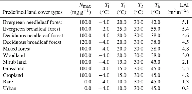
Parameters needed for simulating plant photosynthesis in-clude the maximum foliar N contentNmax(mg g−1), the low (T1)and high (T2)temperature limits for CO2uptake, and the lower (Tl)and upper (Th)ranges of optimum temperature for plant photosynthesis (Table 2). These parameters are used to

2550 G. Tang and P. J. Bartlein: Modifying a DGVM for water-balance simulation

Table 1. Hydrologic relevant parameters for predefined land covers.

LeL f1 Wmin CaC Emax Intc

Predefined land cover types (years) (mm s−1) (mm day−1)

Evergreen needleleaf forest 4.0 0.70 0.0 0.3 5.5 0.04 Evergreen broadleaf forest 2.5 0.80 0.0 0.5 5.5 0.02 Deciduous needleleaf forest 0.5 0.70 0.0 0.3 4.0 0.04 Deciduous broadleaf forest 0.5 0.70 0.0 0.5 4.0 0.02 Mixed forest 0.5 0.70 0.0 0.4 6.0 0.03 Woodland 0.5 0.80 0.0 0.3 4.0 0.02 Shrub land 0.5 0.83 0.1 0.4 5.5 0.02 Grassland 0.5 0.80 0.2 0.5 6.0 0.01 Cropland 0.5 0.80 0.2 0.5 4.5 0.01 Bare 0.5 0.75 0.0 0.0 1.0 0.00 Urban 0.5 0.75 0.0 0.0 0.0 0.00

LeL is short for leaf longevity;f1stands for fraction of roots in soil upper layer. Fraction of roots in soil bottom layer (f2) equals one minusf1;Wminstands for minimum water scalar at which leaves shed by drought deciduous biome; CaC stands for canopy conductance component that is not associated with photosynthesis;Emaxrefers to maximum transpiration rate; Intc stands for interception storage parameter. The specific value of each parameter refers to published research (e.g. Sitch et al., 2003).

Table 2. Photosynthetic relevant parameters for predefined land covers.

Nmax Tl T1 T2 Th LAI

Predefined land cover types (mg g−1) (◦C) (◦C) (◦C) (◦C) (m2m−2)

Evergreen needleleaf forest 100.0 −4.0 20.0 30.0 42.0 5.1 Evergreen broadleaf forest 100.0 2.0 25.0 30.0 55.0 5.4 Deciduous needleleaf forest 100.0 −4.0 20.0 30.0 38.0 4.6 Deciduous broadleaf forest 120.0 −4.0 20.0 30.0 38.0 4.5 Mixed forest 100.0 −4.0 20.0 30.0 38.0 4.8 Woodland 100.0 −4.0 20.0 30.0 38.0 3.0 Shrub land 100.0 −4.0 15.0 30.0 45.0 2.1 Grassland 100.0 −4.0 15.0 30.0 45.0 2.5 Cropland 100.0 −4.0 15.0 30.0 45.0 4.2 Bare 0.0 −4.0 10.0 30.0 45.0 1.3 Urban 0.0 −4.0 10.0 30.0 45.0 0.3

Nmaxis the maximum foliar N content;TlandThare the low and high temperature limits for CO2uptake;T1and T2are the lower and upper ranges of optimum temperature for photosynthesis; LAI is short for leaf area index. The specific value of each parameter except for LAI refers to published work (e.g. Sitch et al., 2003). The LAI for each predefined land cover type refers to the Global Leaf Area Index Data from field measurements compiled at the Oak Ridge National Laboratory Distributed Active Archive Centre (DAAC)

(http://daac.ornl.gov/VEGETATION/lai des.html).

calculate total daytime net photosynthesis of plants and con-vert daytime net photosynthesis into water vapor using an ideal gas equation (Haxeltine and Prentice, 1996), which is later used to simulate canopy conductance (see Eq. 2). The specific value of each parameter refers to published work (e.g. Smith et al., 2001; Sitch et al., 2003).

2.3 Soil water balance in LH

The calculation of each hydrologic variable in LH is almost the same as that described in Gerten et al. (2004). We briefly introduce the calculation of major output variables (Fig. 1) for reference. Daily equilibrium PET rateEeq (mm) is ex-pressed as

Eeq= 1 1+γ×

Rn

L (5)

the Priestley-Taylor coefficient (α)with values that may vary from 1.26 (for well-watered land) to 1.4 (for dry land) is used to estimate potential evapotranspiration (Ep)at different lo-cations as follows:

Ep=Eeq×α. (6)

Actual ET is the sum of interception loss, vegetation tran-spiration, and evaporation from soil. Daily interception loss, L(mm), is a product of daily PET (Ep)and the fraction of day-time,ω(dimensionless), when the canopy is wet is as follows:

L=Ep×ω. (7)

The value ofωis related to the canopy interception storage capacity. Vegetation transpiration is estimated based on the comparison between an atmosphere-controlled demand func-tion and a plant-controlled supply funcfunc-tion (see Eq. 3).

Daily evaporation Ed (mm) from soil follows Huang et al. (1996) as

Ed=Epwr20(1−fvc) (8)

where wr20(dimensionless) represents the relative moisture in the evaporation layer (20 cm) of the soil column; fvc is again the fraction of foliar vegetative cover in a cell, as in Eq. (3).

Daily soil water content in both layers at dayiis updated taking account of the water content from the previous day, snowmeltMi(mm), throughfall Prt(mm), transpirationET,i (mm), evaporationEd,i(mm), percolationp1,i(mm) through two layers, and runoffR1,i(mm) during the current dayi:

1SW1,i=1SW1,i−1+Prt,i+Mi−β1,i×ET,i−Ed,i−p1,i−R1,i

1SW2,i=1SW2,i−1+p1,i−β2,i×ET,i−R2,i−p2,i (9)

where1SW1,i and1SW2,i (mm) are daily changes in soil water content of both layers at dayi;β1 andβ2 represent the fractions of water extracted for transpiration from each layer (β1+β2=1). The surface runoff (R1,i)and subsurface runoff (R2,i)are estimated from the excess of water over field capacity of the two soil layers, respectively. The total runoff in a grid cell is the sum of surface and subsurface runoff.

2.4 Snowmelt computation in LH

Unlike LPJ-DGVM (Sitch et al., 2003; Gerten et al., 2004) which uses a degree-day method for snowmelt calculation, LH combines both the effects of solar radiation and temper-ature on snowmelt (mm) at dayias follows (e.g. Kane et al., 1997):

Mi =

c1×(1−Sal)×dri×dli ifTair< Tsnow

c1×(1−Sal)×dri×dli+c2×(Tair−Tsnow)×Pr (10) if Tair>=Tsnow

where Sal is snow albedo; dri(W m−2h−1)is downward net shortwave radiation flux in dayi; dli (h) is day length in day i; Tair (◦C) is daily air temperature;Tsnow (◦C) is tempera-ture (0◦C) at which snow occurs; Pr (mm) is daily precipita-tion; andc1 andc2 are empirical coefficients. The value of c1 ranges from 0.0002 for grass, crop, and not well-forested land to 0.001 for well-forested land.c2 is set at 0.065 level in LH.

3 Data

3.1 Land cover and soil properties

The global land cover classification from the Global Land Cover Facility (GLCF) at the University of Maryland (http: //glcf.umiacs.umd.edu/data/vcf/) is used to define input land cover at each grid cell that is most likely to exist in the conter-minous US or worldwide. After excluding water, we grouped the rest of 13 GLCF land cover classes into 11 types (Tables 1 and 2). These 11 land cover types were regridded onto both the Parameter-elevation Regressions on Independent Slopes Model (PRISM) 2.5-arc-min elevation points (Daly et al., 2000, 2002) and CRU TS 0.5-degree climate points (Mitchell and Jones, 2005), respectively. Following the same approach, the GLCF Vegetation Continuous Fields (VCF) data (Hansen et al., 2000, 2003) were used to define fraction of foliar veg-etative cover of a GLCF-based land cover in a grid cell. The VCF data contained proportional estimates for three cover types: woody vegetation, herbaceous vegetation, and bare ground. The total percentage cover for three cover types in a cell is 100 percent (Hansen et al., 2000).

Our soil data for the conterminous US were derived from the Miller and White (1998) soil texture classes that were gridded at a 250 m spatial resolution. These soil texture classes were based on the State Soil Geographic (STATSGO) Database, distributed by the United States Department of Agriculture Natural Resources Conservation Service. We re-classified 16 standard soil classes in STATSGO data into eight classes to match those defined in both LH and LPJ-DGVM. The soil data were regridded onto 2.5 arc-min PRISM elevation points. For the global application of LH, we used soil texture data distributed with LPJ-DGVM at a 0.5-degree grid. Annual atmospheric CO2concentrations for both the US and globally were from Schlesinger and Maly-shev (2001).

3.2 Climate data

To apply LH in the US, we used monthly mean tempera-ture (◦C) and precipitation (mm) at 2.5 arc-min grid cells developed by the PRISM Climate Group (Daly et al., 2000, 2002). Monthly percent sunshine (%) and wet-day frequency (days) were derived from the CRU TS 3.0 data sets (Mitchell and Jones, 2005). We interpolated 0.5-degree CRU wet-day frequency data onto the PRISM 2.5-arc-min elevation

2552 G. Tang and P. J. Bartlein: Modifying a DGVM for water-balance simulation

points following the approach described in Tang and Beck-age (2010), in which we first treated climatic value at each CRU grid cell as a function of its latitude, longitude and el-evation to estimate the local lapse rate of wet-day frequency. The calculated local lapse rate was then used to interpolate CRU data to PRISM 2.5 arc-min resolution considering ele-vational differences between CRU and PRISM points. These adjusted climatic values for CRU points were bilinearly in-terpolated onto PRISM points. The CRU sunshine data were downscaled by bilinear interpolation. To apply LH globally, we directly used CRU TS 3.0 monthly mean temperature (◦C), precipitation (mm), percent cloud cover (%), and wet day frequency (days) data on its 0.5-degree grid.

3.3 Reference data and evaluation approaches

Several existing sets of observed or simulated data generated using different methods at different spatial scales were used to test LH’s performance in simulating ET, soil moisture, and surface runoff for the conterminous US (Table 3). The German ET data for the Florida Everglades (US) (German, 2000) was evaluated on the basis of the Bowen-ratio energy budget method (Bowen, 1926). All data needed for applica-tion of the Bowen-ratio method, including net radiaapplica-tion, soil temperature, water level, air temperature, and vapor pres-sure, were measured at 15-min intervals spanning the year from 1996 to 2001 and at nine sites ranging from 24.75◦N to 26.25◦N and from 79.75◦W to 81.25◦W (German, 2000). The V¨or¨osmarty et al. ET data (hereafter V¨or¨osmarty ET, V¨or¨osmarty et al., 1998) were computed by a global-scale water balance model that considered effects of wind speed and vapor pressure on surface hydrology.

Illinois soil-moisture data consisting of total soil moisture were measured at 19 stations in Illinois in the US. These data span an interval from January 1981 to June 2004 and were calibrated with gravimetric observations. We did not use the first three years (1981, 1982 and 1983) for compar-ison because the data have smaller variability than the rest of the record (Hollinger and Isard, 1994). Iowa soil-moisture data consisted of observations from two catchments located at 41.2◦N and 95.6◦W. Each catchment had three sites where soil-moisture observations were made. These observations gave 23 yr of record spanning from 1972 to 1994, but obser-vations were made mostly between April and October (Entin, 1998; Entin et al., 2000). Both Illinois and Iowa soil moisture data are available from the Global Soil Moisture Data Bank (Robock et al., 2000). When necessary, we converted mea-sured soil moisture into millimeters to match LH-simulated moisture levels. We only used soil moisture from the top 50 cm of soil layers because other information, such as soil density for the rest of layers, was not available for unit con-version.

The Global Runoff Data Centre (GRDC) composite runoff fields (CRF) (Fekete et al., 2002) were used to evaluate the spatial pattern of LH-simulated annual runoff for the

conter-minous US. The GRDC CRF was developed by combining observed river discharge information with climate-driven wa-ter balance model outputs. The observed discharge was de-rived from selected gauging stations from the World Meteo-rology Organization GRDC data archive. These station data were coregistered to a simulated topological network at a 0.5-degree land grid.

US Geological Survey (USGS) water data from 13 river gage stations (Table 4) were used to test LH-simulated river stream flow for the years 1981–2006. We selected only 13 rivers for comparison because (i) the derived watersheds from 13 gage stations cover most of the conterminous US (Supplement Fig. S1) and (ii) the observed discharge infor-mation might not always be available for other rivers dur-ing the study period. We converted simulated surface runoff (mm) into cubic meters per second (m3s−1_{)under the} as-sumption that modeled surface runoff at all grid cells inside a watershed flows out of its gage station within the given month. The conversion of modeled surface runoff into stream flow (fLH,j)in monthj is expressed as

fLH,j= 1 n

n

X

i=1

srfi,j×DA/(DSj×86 400)/1000 (11)

where srfi,jis LH-simulated surface runoff (mm) at grid cell iin monthj;nis the number of grid cells inside a watershed; DA is the drainage area (m2)for a gage station; and DSj is the number of days in monthj. We also converted the USGS stream flow data from cubic feet per second into cubic meters per second for comparison.

We used observed river discharges for 10 large rivers worldwide (Tables 3 and 4) to further evaluate LH’s reliabil-ity, largely because the hydrological component from LPJ-DGVM was originally developed for global-scale vegetation and hydrology simulation. We used Cogley (1998) runoff data on a 1-degree grid to evaluate the spatial pattern of LH-simulated annual runoff for the world (Table 3). The global 0.5-degree annual runoff data based on field observations from Fekete et al. (1999) were used to evaluate LH-simulated magnitudes of annual runoff globally and in different latitu-dinal zones (Table 3).

We used statistical measures such as R-squared (R2), root-mean-squared-error (RMSE), and the Nash-Sutcliffe coeffi-cient (Nr)(Nash and Sutcliffe, 1970) to quantify the agree-ment between modeled and simulated/observed ET, soil moisture, and surface runoff. For example, the Nash-Sutcliffe coefficient was used to quantify the agreement between mod-eled and observed stream flow for selected rivers in the con-terminous US.

3.4 Experimental simulations

Table 3. List of observed and simulated data to test LH’s performance.

Testing data list Methods Temporal resolu-tion

Size Data sources∗

(1) German ET (2) V¨or¨osmarty ET

Composite Simulated

Monthly for 1996–2000 Monthly

Plots 0.5◦

German (2000) V¨or¨osmarty et al. (1998) (3) Illinois soil

moisture

Observed Monthly for 1981–2004

Plots Hollinger and Isard (1994) (4) Iowa soil moisture Observed Monthly for

1981–1994

plots Entin (1998), Entin et al. (2000)

(5) The GRDC CRF Composite Annual 0.5◦ Fekete et al. (2002) (6) The USGS water

data

Observed Monthly for 1981–2006

Plots http://waterdata.usgs.gov/ (7) Cogley runoff data Derived Annual 1◦ Cogley (1998)

(8) The Global River Discharge Database

Observed Annual for 1961–1990

Plots http://www.sage.wisc.edu/ riverdata/

(9) Gridded Global Runoff

Observed Annual 0.5◦ Fekete et al. (1999)

∗_{Soil moisture data are available from http://climate.envsci.rutgers.edu/soil moisture/ owned by Robock et al. (2000). The global runoff}

data are available from http://www.grdc.sr.unh.edu/html/Data/index.html.

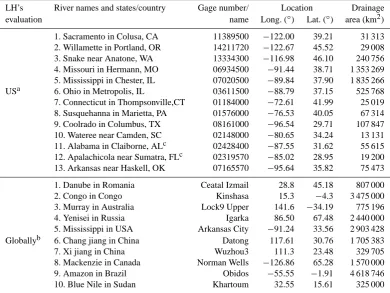
Table 4. Details of river gage stations used for model evaluation in both the US and globally.

LH’s River names and states/country Gage number/ Location Drainage evaluation name Long. (◦) Lat. (◦) area (km2)

1. Sacramento in Colusa, CA 11389500 −122.00 39.21 31 313 2. Willamette in Portland, OR 14211720 −122.67 45.52 29 008 3. Snake near Anatone, WA 13334300 −116.98 46.10 240 756 4. Missouri in Hermann, MO 06934500 −91.44 38.71 1 353 269 5. Mississippi in Chester, IL 07020500 −89.84 37.90 1 835 266 USa 6. Ohio in Metropolis, IL 03611500 −88.79 37.15 525 768 7. Connecticut in Thompsonville,CT 01184000 −72.61 41.99 25 019 8. Susquehanna in Marietta, PA 01576000 −76.53 40.05 67 314 9. Coolrado in Columbus, TX 08161000 −96.54 29.71 107 847 10. Wateree near Camden, SC 02148000 −80.65 34.24 13 131 11. Alabama in Claiborne, ALc 02428400 −87.55 31.62 55 615 12. Apalachicola near Sumatra, FLc 02319570 −85.02 28.95 19 200 13. Arkansas near Haskell, OK 07165570 −95.64 35.82 75 473 1. Danube in Romania Ceatal Izmail 28.8 45.18 807 000 2. Congo in Congo Kinshasa 15.3 −4.3 3 475 000 3. Murray in Australia Lock9 Upper 141.6 −34.19 775 196 4. Yenisei in Russia Igarka 86.50 67.48 2 440 000 5. Mississippi in USA Arkansas City −91.24 33.56 2 903 428 Globallyb 6. Chang jiang in China Datong 117.61 30.76 1 705 383 7. Xi jiang in China Wuzhou3 111.3 23.48 329 705 8. Mackenzie in Canada Norman Wells −126.86 65.28 1 570 000 9. Amazon in Brazil Obidos −55.55 −1.91 4 618 746 10. Blue Nile in Sudan Khartoum 32.55 15.61 325 000

a_{The river gage stations are based on USGS National Water Information System (http://waterdata.usgs.gov/nwis/);}b_{the river gage stations}

worldwide are based on the Global River Discharge Database (http://www.sage.wisc.edu/riverdata/).cThe Alabama and Apalachicola River watersheds are combined together for reference as the Alabama River watershed.

2554 G. Tang and P. J. Bartlein: Modifying a DGVM for water-balance simulation

atmospheric CO2concentration (650 ppm). Results from the first simulation were compared to the simulation under the consideration of both temperature and solar radiation ef-fects on snowmelt and actual atmospheric CO2 concentra-tion. Results from the second simulation were compared to the simulation run under low atmospheric CO2 concentra-tion (360 ppm). Such comparisons aimed to evaluate how the addition of solar radiation effect on snowmelt impacts mod-eled river stream flow and how increasing atmospheric CO2 concentration affects modeled actual evapotranspiration.

4 Results

4.1 LH-simulated actual ET and its evaluation in the US

LH-simulated annual actual ET averaged 536 mm in the US and varied from 0 to 1305 mm among grid cells (Fig. 2a). The lowest ET was simulated in southeastern California where annual precipitation is low (<160 mm) and temperature is high (>21◦C) (Supplement Fig. S2). The highest ET was simulated in coastal areas of the southern and southeastern US where both annual precipitation (>1400 mm) and tem-perature (>20◦C) are high. In the eastern US, annual ET was simulated to decrease from south to north (Fig. 2a), a re-sult of energy- and temperature-related latitudinal gradients (Supplement Fig. S2). In the western US, annual ET was less than 600 mm in most areas and did not vary much latitudi-nally. In some mountain ranges of the western US, such as the (Pacific) Coast Range, simulated annual ET ranged from 600 to 900 mm (Fig. 2a), attributed to high annual precipita-tion (>2600 mm) in these areas (Supplement Fig. S2).

The magnitudes of LH-simulated annual ET among grid cells agreed well with those from V¨or¨osmarty ET data (V¨or¨osmarty et al., 1998). For example, the simulated mean annual ET (533 mm) was close to 572 mm from V¨or¨osmarty ET. The range (0 to 1305 mm) of LH-simulated annual ET was similar to the range of 53 to 1414 mm of V¨or¨osmarty ET data. The standard deviation of LH-simulated annual ET was 238 mm, close to the 269 mm from V¨or¨osmarty ET data. The spatial pattern of LH-simulated ET (Fig. 2a) agrees well visu-ally with that depicted by the V¨or¨osmarty ET data (Fig. 2b). In the eastern US, for instance, annual ET decreased from more than 1200 mm in the south to below 600 mm in the north in both the simulated and V¨or¨osmarty ET data. In the western US, annual ET varied from 0 to 600 mm in most ar-eas except for mountain ranges (Fig. 2).

When averaged for all grid cells in a watershed, LH-simulated monthly ET was strongly correlated (R2>0.72, p<0.01) with values from V¨or¨osmarty ET data in 12 large watersheds (Fig. 3 and Table 5), indicating that LH cap-tured well the variation in monthly ET illustrated in the V¨or¨osmarty ET data. Average monthly ET (based on a 12-month mean) under the LH simulation was close (difference <10 %) to those from V¨or¨osmarty ET data respectively in

46 Figures

970 971

Figure 1 972

973

974 975 976 977

Figure 2 978

979

980 981 982 983

Fig. 2. (a) The LH-simulated 26-yr (1981–2006) average annual

actual ET at 2.5 arc-min grid cells; (b) annual actual ET from V¨or¨osmarty et al. (1998) at 0.5-degree grid cells. The white areas in (a) and (b) are water excluded for simulation.

the Sacramento, Snake, Missouri, Mississippi, Ohio, Con-necticut, Susquehanna, Colorado, and Arkansas watersheds (Table 5). Major differences occurred in estimates of monthly ET for the Willamette, Alabama, and Wateree watersheds, in which LH-simulated monthly ET was 19 % higher, 16 % lower, and 20 % lower than V¨or¨osmarty monthly ET, respec-tively (Table 5). In more detail, LH-simulated ET in late spring and early summer in most watersheds was smaller than those from V¨or¨osmarty ET data (Fig. 3).

Table 5. Comparison between LH-simulated and V¨or¨osmarty et al. ET (V¨or¨osmarty et al., 1998) data in12 major river watersheds in the US.

V¨or¨osmarty et al. ET (mm) LH-simulated ET (mm) Statistics Rivers min max mean min max mean R2 1(%) 1. Sacramento 6 90 37 12 64 38 0.72 0.6 2. Willamette 7 83 43 7 100 51 0.94 19.3 3. Snake 1 91 27 6 53 29 0.76 7.5 4. Missouri 0 118 41 6 69 37 0.88 −10.0 5. Mississippi∗ 0 132 55 6 108 51 0.88 −5.8 6. Ohio 0 125 61 8 116 58 0.88 −4.6 7. Connecticut 0 111 43 2 120 40 0.81 −6.3 8. Susquehanna 0 110 46 4 124 46 0.86 −0.6 9. Colorado 12 73 48 28 70 48 0.79 −0.4 10. Wateree 0 135 78 15 110 66 0.85 −15.8 11. Alabama 30 138 90 22 113 72 0.90 −20.1 12. Arkansas 0 104 47 13 71 44 0.86 −6.8

∗_{The observed monthly stream flow subtracted that from the Missouri River in model comparison.}

47

Figure 3

984

985

986

987

988

989

990

Figure 4

991

992

993

994

Figure 5

995

996

997

Fig. 3. Comparison between LH-simulated (solid line) and V¨or¨osmarty et al. monthly ET (V¨or¨osmarty et al., 1998) (dashed line) in the 12

river watersheds.

47 Figure 3

984 985

986 987 988 989 990

Figure 4 991

992 993 994

Figure 5 995

996

997

Fig. 4. Comparison between LH-simulated (black line) to observed

(dashed line) monthly ET (German, 2000) during the years 1996– 2001 in Florida Everglades (US).

4.2 LH-simulated soil moisture and its evaluation in the US

LH-simulated annual soil moisture averaged 107 mm over the US and ranged from 0 to 325 mm among grid cells (Fig. 5). Annual soil moisture was simulated to be high-est in mountain areas, such as the Pacific Coast Ranges, the Cascade Range of Oregon, and the Appalachian Moun-tains in the eastern and northeastern US (Fig. 5). In these areas, LH-simulated annual soil moisture exceeded 160 mm, attributable to low regional annual temperature (<9◦C) and high precipitation (>1500 mm). Annual soil moisture was simulated to be low (<100 mm) in most of the western US. In these regions, annual precipitation was relatively low (<400 mm) while annual mean temperature can be more than 9◦C (Supplement Fig. S2).

2556 G. Tang and P. J. Bartlein: Modifying a DGVM for water-balance simulation

47 Figure 3

984 985

986 987 988 989 990

Figure 4 991

992 993 994

Figure 5 995

996

997

Fig. 5. LH-simulated 26-yr (1981–2006) mean annual soil moisture

in the top 50 cm of soil layers.

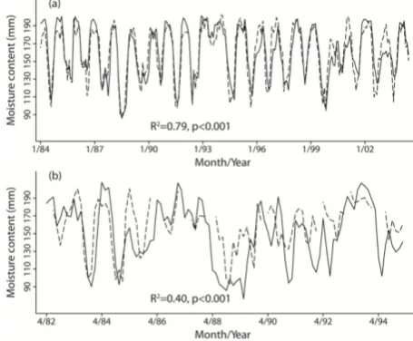
When LH-simulated monthly soil moisture was compared to Illinois soil moisture (Table 3), the statistics (R2=0.79, p<0.01) suggest that LH captured well the variation in monthly soil moisture in this region during the years 1984– 2001 (Fig. 6a). The LH-simulated monthly soil moisture av-eraged 160 mm, equaling 160 mm from observed data. LH-simulated monthly mean value ranged from 87 to 202 mm during the period 1984–2001, resembling observed values ranging from 86 to 201 mm. The standard deviation of LH-simulated soil moisture was 29.3 mm, close to 28.9 mm from the observations. The RMSE between LH-simulated and ob-served values for 246 months was 14, indicating that LH simulated well monthly soil moisture in this region though it under- and overestimated soil moisture in some months (Fig. 6a).

Additional comparison against observed soil moisture in two Iowa catchments (Table 3) still suggested that LH can capture the variation of monthly soil moisture at local scales as indicated by the coefficient (R2=0.40,p<0.01) between the two data sets (Fig. 6b). For the whole period 1981–2004, LH-simulated monthly soil moisture averaged 149 mm, only 10 mm lower than the average from observed data (159 mm). LH-simulated monthly soil moisture ranged from 76 to 208 mm, a slightly broader range than observed values (93 to 201 mm). Nevertheless, LH-simulated soil moisture in this particular region was comparatively more variable than ob-served values, as indicated by the standard deviations of 26 mm for LH and 34 mm for observation. The RMSE be-tween LH-simulated and observed values for 91 points was 29, accounting for 18 % of observed mean monthly soil mois-ture.

4.3 LH-simulated surface runoff and its evaluation in

the US

LH-simulated annual surface runoff averaged 234 mm in the US and ranged between 0 and 6440 mm among grid cells,

48 Figure 6

998

999 1000

Figure 7 1001

1002

Fig. 6. Comparison between LH-simulated (black line) and

ob-served (dashed line) soil moisture in the top 50 cm of soil layers in (a) Illinois in the US during the years 1984–2004 (Hollinger and Isard, 1994), and (b) Iowa in the US during the years 1981–1994 (Entin, 1998; Entin et al., 2000). For Illinois soil moisture, only half year (till June) data for 2004 are available. LH-simulated soil mois-ture in Illinois was averaged for all grid cells ranging from 91.25◦W to 88.25◦W and from 37.25◦N to 42.25◦N; a spatial extent that ap-proximately matches the extent of Illinois soil moisture. Measured soil moisture in Iowa was not available for some months and years, but most records were available between April and October.

with a standard deviation of 307 mm (Fig. 7a). As was the case for annual soil moisture, surface runoff was simulated to be highest in mountain areas. In these regions, annual precip-itation was comparatively high while annual mean tempera-ture was comparatively low (Supplement Fig. S2). Annual surface runoff was modeled to be low in most of the west-ern US, attributed to low annual precipitation (<400 mm). Overall, LH-simulated surface runoff was more than 200 mm in the eastern US but less than 200 mm in the western US (Fig. 7a).

G. Tang and P. J. Bartlein: Modifying a DGVM for water-balance simulation 2557

48 Figure 6

998

999 1000

Figure 7 1001

1002

Fig. 7. (a) The LH-simulated annual surface runoff at 2.5 arc-min

grid cells and (b) the GRDC composite annual runoff at 0.5-degree grid cells (Fekete et al., 2002) for the conterminous US.

deviations of LH-simulated surface runoff (307 mm) and the GRDC CRF data (278 mm).

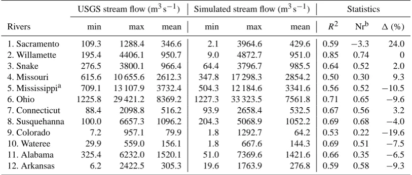
Further comparison of LH-simulated monthly stream flow to the USGS water data demonstrated that LH was able to correctly simulate the variations in monthly stream flow in most major rivers in the US (R2>0.50, p<0.01; Nr>0.51, Moriasi et al., 2007) (Fig. 8). Especially for water-sheds where forest is the dominant land cover (Supplement Fig. S3), the LH-simulated monthly stream flow agreed well (R2>0.65,p<0.01; Nr>0.52) with observed values for the years 1981–2006. These rivers include the Willamette, Ohio, Susquehanna, Connecticut, and Wateree (Fig. 8 and Table 6). In contrast, for watersheds where grass, shrubs and/or crops are dominant land covers, the agreement between compared data was weaker (R2<0.65). These rivers include the Snake, Missouri, Mississippi, and Colorado, but not the Arkansas River for which the modeled monthly stream flow agreed well with the observed stream flow (Fig. 8 and Table 6).

The magnitudes of LH-simulated mean monthly stream flow for the years 1981–2006 were close (difference<11 %) to measured mean monthly stream flow for most of the 12 rivers, including the Willamette, Snake, Missouri, Missis-sippi, Ohio, Connecticut, Susquehanna, Wateree, and Al-abama (Table 6). Major difference occurred in estimates of monthly mean stream flow for the Sacramento and Colorado River. For these two rivers, LH-simulated average monthly

stream flow was 24.0 % higher and 19.6 % lower than their counterparts from measured data, averaging 347 and 80 m3s−1_{, respectively (Table 6). Although LH-simulated} mean monthly flow was similar to observed values in most rivers, it was more variable than measured values for most rivers during the years 1981–2006 as indicated by the min-imum and maxmin-imum monthly stream flows between com-pared data sets (Table 6).

4.4 LH-simulated river discharge and its evaluation

globally

For the global land surface as a whole, LH-simulated long-term (1961–1990) mean annual surface runoff averaged 292 mm, only 30 mm less than that (322 mm) in the Cog-ley (1998) annual runoff data. The standard deviation of LH-simulated mean annual surface runoff among 59 199 grids cells was 438 mm, almost equaling 442 mm from Cogley runoff data. The spatial patterns of LH-simulated mean an-nual surface runoff for the entire world visually agreed well with those of Cogly runoff data (Fig. 9a and b). For exam-ple, both data showed that mean annual surface runoff was less than 100 mm in most parts of the western China, central Asia, and the western US, where semi-arid and arid ecosys-tems dominate. In contrast, both data sets showed that mean annual surface runoff in the Amazon and Congo River basins, southeastern Asia, and the eastern part of North America were more than 500 mm (Fig. 9a and b).

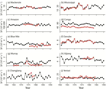
The magnitudes of LH-simulated mean annual discharges for 10 large rivers worldwide were generally in good agree-ment with observed values for these rivers (Table 7). For ex-ample, LH-simulated mean annual discharge almost equaled (difference <1 %) observed values for the Danube River in Europe, the Mackenzie River in North America, and the Amazon River in South America (Table 7). In addition, LH-simulated mean annual discharge was only 8 %, 5 %, and 15 % less than observed values for the Yenisei River in Rus-sia, the Xi Jiang River and Chang Jiang River in China, re-spectively. It was only 6 % higher than the observed value for the Mississippi River in the US. Large differences oc-curred for the Congo River and Blue Nile River in Africa, and the Murray River in Australia. For these large rivers, LH-simulated mean annual discharge was about 60 % (for the two African rivers) and 199 % higher (for the Murray River) than observed values, respectively (Table 7). LH also captured well (R2>0.37,p<0.01) interannual variations of river discharges for most large rivers, including the Macken-zie, Mississippi, Danube, Chang Jiang, Amazon, and Mur-ray River (Fig. 10). When aggregated by 1◦latitudinal zones, LH-simulated mean annual surface runoff was in accordance with previously published data (Fig. 11), but LH slightly overestimated annual surface runoff between 0◦S and 15◦S latitudinal zones and underestimated it between 25◦N and 35◦N latitudinal zones.

2558 G. Tang and P. J. Bartlein: Modifying a DGVM for water-balance simulation

49

Figure 8

1003

1004

1005

1006

1007

1008

1009

1010

1011

1012

1013

1014

1015

1016

1017

1018

1019

1020

1021

1022

Fig. 8. Comparison between LH-simulated (red line) and US Geological Survey observed monthly stream flow (SF) (black line) at 12 river

gage stations. Nr is the Nash-Sutcliffe coefficient.

Table 6. Comparison between LH-simulated and observed stream flow for 12 major rivers in the US.

USGS stream flow (m3s−1) Simulated stream flow (m3s−1) Statistics Rivers min max mean min max mean R2 Nrb 1(%) 1. Sacramento 109.3 1288.4 346.6 2.1 3964.6 429.6 0.59 −3.3 24.0 2. Willamette 195.4 4406.1 950.7 9.0 4872.7 951.0 0.85 0.74 0 3. Snake 276.5 3800.1 966.4 64.4 3796.7 985.5 0.64 0.52 2.0 4. Missouri 615.6 10 655.6 2612.3 347.8 17 298.3 2854.2 0.50 0.30 9.3 5. Mississippia 709.1 13 107.9 3732.4 504.3 12 184.6 3341.6 0.56 0.52 −10.5 6. Ohio 1225.8 29 421.2 8369.2 1227.3 33 323.5 7561.8 0.71 0.65 −9.6 7. Connecticut 88.4 2098.8 516.2 93.9 2658.4 532.5 0.67 0.56 3.2 8. Susquehanna 100.0 6657.3 1096.2 204.3 5068.9 1052.2 0.69 0.68 −4.0 9. Colorado 7.2 957.1 79.9 1.8 1292.7 64.2 0.53 0.22 −19.6 10. Wateree 29.9 559.0 156.1 1.8 667.6 144.3 0.69 0.51 −7.5 11. Alabama 325.4 6232.0 1520.1 51.0 7369.6 1421.6 0.66 0.35 −6.5 12. Arkansas 6.2 2422.5 305.3 19.6 1763.9 276.8 0.59 0.58 −9.3

Table 7. Comparison between LH-simulated and observed annual discharges for 10 large rivers worldwide.

Compare period Observed discharge (m3s−1) Simulated discharge (m3s−1) Diff (%) Rivers Fist year Last year min max mean min max mean

1. Danube 1961 1984 5219 9293 6838 3314 9360 6790 −1 2. Congo 1961 1983 34 690 54 964 43 403 58 385 97 492 69 723 61 3. Murray 1965 1984 36 1108 257 283 1826 769 199 4. Yenisei 1961 1984 11 584 20 966 17 570 36 1108 16 232 −8 5. Mississippi 1961 1979 9884 25 993 16 574 9884 25 993 17 488 6 6. Chang jiang 1976 1979 23 728 31 770 25 032 17 000 26 049 21 255 −15 7. Xi jiang 1976 1983 6607 8311 7085 5905 7977 6735 −5 8. Mackenzie 1967 1984 7191 9662 8343 7433 10 185 8436 1 9. Amazon 1972 1982 138 608 176 067 165 615 145 992 207 499 176 073 0 10. Blue Nile 1976 1990 805 2436 1528 1695 3344 2539 66

4.5 Results of two experimental simulations

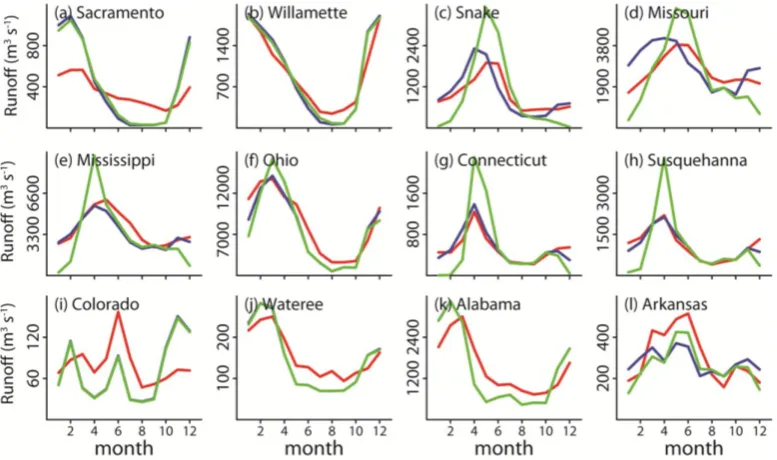
LH-simulated monthly stream flow in winter and early spring with the addition of radiation effect on snowmelt was closer than the degree-day method to observed values in the Snake, Missouri, Mississippi, Ohio, Connecticut, and Susquehanna watersheds (Fig. 12c–h). In these watersheds, heavy snow of-ten occurs in winter and early spring. Because less snowmelt was simulated under the degree-day method in winter and early spring, the subsequent monthly stream flow was much higher than observed values in late spring in these watersheds where heavy snow occurs in winter and spring (Fig. 12c– h). For the Alabama, Wateree and Colorado River (Fig. 12i– k), the simulated stream flows under the two approaches were almost identical because temperature is relatively high (>0◦C) in winter and heavy snow rarely occurs in these wa-tersheds.

LH-simulated annual ET under high CO2 concentration was about 30 to 75 mm lower than ET values simulated un-der low CO2 concentration in watersheds where forests are dominant land covers. The reason is because the higher CO2 concentration induced plant stomatal closure and thus de-creased plant transpiration by a range of 33 to 73 mm in forest-dominated watersheds, such as the Connecticut and Susquehanna watersheds.

5 Discussion

Although model evaluation suggests LH performs well, much effort is still needed to improve the accuracy in simulating land-surface water balances. For example, LH-simulated monthly ET in summer was less than the V¨or¨osmarty ET data in the Snake, Missouri, Mississippi and Arkansas watersheds (Fig. 3). In the Midwestern and western US, relative atmospheric humidity is comparatively lower than watersheds in the eastern and southern US. Actual ET is considered to increase as vapor-pressure deficit increases. V¨or¨osmarty et al. (1998) considered the effects of relative

hu-50 Figure 9

1023

1024 1025 1026 1027 1028 1029 1030 1031 1032 1033 1034 1035 1036 1037

Fig. 9. Long-term mean annual surface runoff (mm): (a)

LH-simulated runoff for the period 1961–1990, (b) observed runoff (Cogley, 1998) for different time periods, (c) difference between LH-simulated and Fekete et al. (1999) runoff data. The 10 large river watersheds in (c) were derived from HydroSHEDS data (Lehner et al., 2006). The geographic location of each gage station was based on Global River Discharge Database (RivDis2.0), avail-able from http://www.sage.wisc.edu/riverdata/. For comparison, we regridded 1-degree Cogley runoff data onto simulated 0.5-degree grids using the nearest neighbor algorithm.

2560

_{Figure 10}

1038

1039

1040

1041

1042

1043

Figure 11

1044

1045

1046

1047

1048

1049

1050

1051

1052

1053

Fig. 10. Comparison between LH-simulated (black dotted line) and observed (red dotted line) annual discharges for 10 large rivers worldwide.

The observed annual discharges are from RivDis2.0 database, available from http://www.sage.wisc.edu/riverdata/.

51 Figure 10

1038 1039

1040 1041 1042 1043

Figure 11 1044

1045

1046 1047 1048 1049 1050 1051 1052 1053

Fig. 11. Estimates of long-term mean annual surface runoff (mm),

aggregated into 1-degree latitude zones. LH-simulated data are 30-yr (1961–1990) long-term mean. The Cogley (1998) runoff data were at 1-degree land grid, and Fekete et al. (1999) runoff data were at 0.5-degree land grid.

midity and vapor pressure deficit on land surface hydrology. This explains why LH-simulated monthly ET in summer was smaller than V¨or¨osmarty ET for those watersheds located in the Midwestern and western US. The consideration of

rela-tive humidity and vapor-pressure deficit in V¨or¨osmarty ET algorithm also contributed to the higher ET estimates in the Wateree and Alabama watersheds (Fig. 3j and k), in which water is not limited but annual mean temperature is high. In the Willamette River watershed, V¨or¨osmarty ET peaked in April and then tended to decrease throughout the rest of year (Fig. 3b), resulting in lower ET simulation although water is not limited in this region. At its current stage, LH considers only radiative forcing while ignoring other meteorological effects on actual ET. Meteorological factors, such as relative humidity, play an important role in determining actual ET (Brunel et al., 2006; Rim et al., 2008), which suggests that they be considered in LH’s future development.

LH-simulated soil moisture in the top 50 cm of the soil layer in US. Illinois and Iowa generally agreed well with ob-served values (Fig. 6). This good agreement indicated that LH has a strong ability to simulate soil moisture at the re-gional or even local scale. In addition, we suspect that the accuracy of input land covers, the 2.5 arc-min PRISM cli-mate data, and the quality of STATSGO soil data, all con-tributed to the good agreement between simulated and ob-served soil moisture in these two regions. Illinois soil mois-ture was monitored at grass-covered sites across Illinois, an agricultural region (Hollinger and Isard, 1994). The GLCF data defines land covers in Illinois as a mix of grass and crops

G. Tang and P. J. Bartlein: Modifying a DGVM for water-balance simulation 2561

52

Figure 12

1054

1055

Fig. 12. Monthly river runoff simulated by LH (a) under the addition of solar radiation for snowmelt computation (blue line), and (b) using

a degree-day method for snowmelt computation (green line), and (c) USGS observed average monthly runoff (red line) for 12 major rivers in the US.

(Supplement Fig. S3). Finer-scale climate data can better rep-resent the spatiotemporal variation of climate across a region. Liu and Yang (2010) suggested that finer-scale climate data are likely to better capture the spatial variation of hydrolog-ical variables than those simulated at coarser resolution. Ac-curate spatial representation of soil moisture is difficult for large areas because it requires consideration of detailed soil attributes such as soil texture and its water holding capacity (Hollinger and Isard, 1994). The STATSGO soil texture data were created by generalizing more detailed soil survey maps and are often thought to be of high quality in representing soil characteristics in the US. Anderson et al. (2006) found that the hydrological simulation can be improved by combining detailed land cover with STATSGO soil data to refine model parameter estimates.

The good agreement between LH-simulated and observed stream flow for major rivers in the US (Fig. 8) and large rivers worldwide (Fig. 10) supports the utility and reliabil-ity of incorporating satellite data into LPJ-DGVM to simu-late land surface water balances. The LH-simusimu-lated spatial pattern of mean annual surface runoff for the entire world was also visually remarkably similar to that captured by LPJ-DGVM (Fig. 2 in Gerten et al., 2004) because the core hy-drologic components in two models are almost the same. On average, LH-simulated global long-term (1961–1990) mean annual surface runoff was 292 mm, only 14 mm less than the LPJ-DGVM simulated runoff (≈306 mm) (Gerten et al., 2004). However, LH-simulated global mean annual surface runoff was much smaller than LPX-simulated surface runoff

(≈444 mm), which tended to overestimate surface runoff magnitude in the tropics and throughout much of the North-ern Hemisphere (Murray et al., 2011). Overall, LH captured well the global runoff distribution (Fig. 9a and b) although it over- and underestimated surface runoff in some areas when compared to observed data from Fekete et al. (1999) (Fig. 9c). For example, like LPJ-DGVM (Gerten et al., 2004), LH tended to underestimate surface runoff in subarctic re-gions. In addition, like LPJ-DGVM (Gerten et al., 2004) and LPX (Murray et al., 2011), LH represented well interannual variations in large river discharges (Fig. 10).

Vegetation and crops are far from static and have important effects on land surface water balance (Arora, 2002). Different vegetation and crops have varying physiological traits, such as LAI and stomatal conductance, affecting plant transpira-tion and soil evaporatranspira-tion due to changes in surface albedo. The accuracy of land cover and soil representation may cause LH-simulated water balances not to agree well with corre-sponding observed values. For example, LH-simulated ET in April of 1998 in the Florida Everglades decreased sharply relative to March and was much lower than the measured value (Fig. 4). Land covers in the Florida Everglades are mostly wetlands that never dry or dry only during parts of years (German, 2000). In contrast, LH (actually the GCLF data) defines land cover in this area as grassland. As a result, precipitation in April could be very low (average 14 mm) while soil evaporation remains high resulting in a higher ET measurement, which suggests the accurate representation of

2562 G. Tang and P. J. Bartlein: Modifying a DGVM for water-balance simulation

land characteristics is required in applying LH at the small regional scale.

The type of land cover affects the accuracy of modeled land-surface water balances. LH better captured the mag-nitudes and variations of monthly stream flow in forest-dominated watersheds relative to those watersheds domi-nated by crops, grassland, or shrubs (Table 6 and Supplement Fig. S3); largely because monthly precipitation was gener-ally higher throughout the year and the hydrologic effects of human activities such as irrigation were comparatively lower in these watersheds. In contrast, for semi-arid and arid en-vironments in the western US and other parts of the world, precipitation is thought to be important for controlling snow or rainfall dominated river hydrography. Excessive soil wa-ter may percolate into deep ground wawa-ter and then discharge in valleys at lower elevations. As a result, actual river peak flow could be lower than LH-simulated flow, such as in the Colorado River through Texas (Fig. 8i).

Like LPJ-DGVM (Gerten et al., 2004), LH does not simu-late human withdrawal of water from rivers and the reduction of river flow by human water consumption (e.g. D¨oll et al., 2003). It is not surprising, therefore, that the magnitudes of LH-simulated monthly stream flow were much higher than observed data for the Sacramento River (Fig. 8a). The Sacra-mento River watershed has been intensely developed for wa-ter supply and hydroelectric power generation. An earlier study (Yates et al., 2009) that considered consumptive and non-consumptive use of water in the Sacramento River wa-tershed was able to correctly reproduce the water balance and river hydrology in the watershed. Likewise, both LH and LPJ-DGVM ignore evaporation loss from lakes, reser-voirs, wetlands, and non-perennial ponds. These processes contributed to overestimation of discharges for large rivers, such as the Murray River and Blue Nile River, in arid regions (Fig. 10) (Gerten et al., 2004). The exclusion of water evap-oration from river channels and potential underestimation of rainfall interception by tropic forest canopies (e.g. Murray et al., 2011) contributed LH-simulated river discharges to be higher than observed values for the Congo River in Africa (Fig. 10d). In addition, the difference between satellite-based land cover and the DGVM-simulated vegetation, the exclu-sion and incluexclu-sion of vegetation-related biogeochemical pro-cesses in the model’s construction, and the setup of model running (e.g. the length of years used for spin-up simula-tion) can affect the agreement between LH- and LPJ-DGVM-simulated water balance in each basin. Further study is there-fore required to explicitly examine how these differences af-fect simulated water balances.

Despite a number of discrepancies that emerged when comparing LH-simulated to observed values of three hydro-logic values at different spatial scales, LH offers several ad-vantages over the use of a standard DGVM for simulating re-gional or global land-surface hydrology. First, LH predefines land covers instead of simulating them as, for example, in LPJ-DGVM. This greatly simplifies LH’s structure (Fig. 1)

but does not reduce LH’s ability to simulate land surface wa-ter balances. This simplification of model structure makes LH easier to grasp (e.g. Paola, 2011). Second, LH ignores some vegetation-related biogeographical and biogeochemi-cal dynamics. Vegetation-related parameters (Tables 1 and 2) are reduced by more than half compared to those in LPJ-DGVM. The reduction of parameters makes LH easier to pa-rameterize in practice. This in turn has potential to reduce the uncertainty of model results resulting from model parame-terization (e.g. Zaehle et al., 2005; Wramneby et al., 2008). Third, the addition of solar radiation for snowmelt computa-tion in LH greatly improved estimates of river stream flow in winter and early spring in snow-dominated watersheds (Fig. 12). Gerten et al. (2004) suggested that LPJ-DGVM tended to underestimate surface runoff in winter at high lat-itudes of the Northern Hemisphere. With the addition of the solar radiation effect on snowmelt, LH-simulated mean an-nual river discharges agreed well with observed values for the Mackenzie and Yenisei Rivers (Fig. 10a and j). Fourth, LH couples plant photosynthesis and phenology. It is there-fore able to simulate the role of changes in atmospheric CO2 concentration in land-surface water balance (e.g. Leipprand and Gerten, 2006; Robock and Li, 2006). The coupling of plants photosynthesis and phenology is also crucial for study-ing effects of land cover change on the land-surface water balance because of the interactions between vegetation and water (e.g. Kergoat et al., 2002; Rost et al., 2008).

6 Conclusions

LH is developed by incorporating satellite-based land covers and proportional foliar vegetation covers into LPJ-DGVM (Sitch et al., 2003; Gerten et al., 2004) for simulating land surface water balances at the regional scale. LH’s perfor-mance has been evaluated at different spatial scales using a compilation of existing data sets. This study concluded the following:

1. LH is able to accurately simulate ET, soil moisture, and surface runoff at the regional scale. The incorporation of satellite-based data into LH helps simplify the model’s structure and thus makes LH easier to grasp. The reduc-tion of model parameters enables LH easier to parame-terize in practice than common DGVMs.

3. Hydrologic evaluation of LH at the regional scale indi-cated that it also has a strong ability to simulate regional scale land surface water balances, but accurate estimates of regional scale land surface hydrology require both LPJ-DGVM and LH to correctly and explicitly define the land characteristics. In addition, human-related fac-tors such as water withdrawal and consumption, meteo-rological factors such as vapor pressure deficit, and the routing of water among simulated units should be con-sidered in LH’s future development.

Supplementary material related to this article is

available online at: http://www.hydrol-earth-syst-sci.net/ 16/2547/2012/hess-16-2547-2012-supplement.pdf.

Acknowledgements. Research was supported by NSF EPSCoR

grant (NSF Cooperative Agreement EPS-0814372), NSF grant number ATM 0602409, and the Department of Geography at the University of Oregon. We greatly appreciate all developers of the Lund-Potsdam-Jena (LPJ) dynamic global vegetation model, with special thanks to Dieter Gerten for developing the surface-hydrology model embedded in LPJ-DGVM. We thank three anonymous reviewers for their valuable comments on this study. We appreciate Sony Pradhanang for her discussion on USGS stream flow data.

Edited by: J. Liu

References

Anderson, R. M., Koren, V. I., and Reed, S. M.: Using SSURGO data to improve Sacramento Model a priori parameter estimates, J. Hydrol., 320, 103–116, 2006.

Arora, V.: The use of the aridity index to assess climate change ef-fect on annual runoff, J. Hydrol., 265, 164–177, 2002.

Arora, V. and Boer, G.: The temporal variability of soil moisture and surface hydrological quantities in a climate model, J. Climate., 19, 5875–5888, 2006.

Betts, R. A., Boucher, O., Collins, M., Cox, P. M., Falloon, P. D., Gedney, G., Hemming, D. L., Huntingford, C., Jones, C. D., Sex-ton, D. M. H., and Webb, M. J.: Projected increase in continental runoff due to plant responses to increasing carbon dioxide, Na-ture, 448, 1037–1041, 2007.

Boegh, E., Thorsen, M., Butts, M. B., Hansen, S., Christiansen, J. S., Abrahamsen, P., Hasager, C. B., Jensen, N. O., van der Keur, P., Refsgaard, J. C., Schelde, K., Soegaard, H., and Thomsen, A.: Incorporating remote sensing data in physically based distributed agro-hydrological modeling, J. Hydrol., 287, 279–299, 2004. Bowen, I. S.: The ratio of heat losses by conduction and by

evap-otranspiration from any water surface, Phys. Rev., 27, 779–787, 1926.

Brabson, B. B., Lister, D. H., Jones, P. D., and Palutikof, J. P.: Soil moisture and predicted spells of extreme temperatures in Britain, J. Geophys. Res., 110, D05104, doi:10.1029/2004JD005156, 2005.

Brovkin, V., van Bodegom, P. M., Kleinen, T., Wirth, C., Cornwell, W. K., Cornelissen, J. H. C., and Kattge, J.: Plant-driven variation in decomposition rates improves projections of global litter stock distribution, Biogeosciences, 9, 565–576, doi:10.5194/bg-9-565-2012, 2012.

Brunel, J. P., Ihab, J., Droubi, A. M., and Samaan, S.: Energy bud-get and actual evapotranspiration of an arid oasis ecosystem: Palmyra (Syria), Agr. Water Manage., 84, 213–220, 2006. Campo, L., Caparrini, F., and Castelli, F.: Use of multi-platform,

multi-temporal remote-sensing data for calibration of a dis-tributed hydrological model: an application in the Arno basin, Italy. Hydrol. Process., 20, 2693–2712, 2006.

Cogley, J. G.: GGHYDRO – Global Hydrographic Data, Release 2.2. Trent Climate Note 98-1. Department of Geography, Trent University, Peterborough, Ontario, Canada, 1998.

Daly, C., Taylor, G. H., Gibson, W. P., Parzybok, T. W., Johnson, G. L., and Pasteris, P.: High-quality spatial climate data sets for the United States and beyond, T. Am. Soc. Agri. Eng., 43, 1957– 1962, 2000.

Daly, C., Gibson, W. P., Taylor, G. H., Johnson, G. L., and Pasteris, P.: A knowledge-based approach to the statistical mapping of cli-mate, Clim. Res., 22, 99–113, 2002.

D¨oll, P., Kaspar, F., and Lehner, B.: A global hydrological model for deriving water availability indicators: model running and val-idation, J. Hydrol., 270, 105–134, 2003.

Engstrom, R., Hope, A., Kwon, H., Harazono, Y., Mano, M., and Oechel, W.: Modeling evapotranspiration in Arctic coastal plain ecosystems using a modified BIOME-BGC model, J. Geophys. Res-Biogeo., 111, G02021, doi:10.1029/2005JG000102, 2006. Entin, J. K.: Spatial and temporal scales of soil moisture

varia-tions. Ph.D. dissertation, Department of Meteorology, University of Maryland, 125 pp. 1998.

Entin, J. K., Robock, A., Vinnikov, K. Y., Hollinger, S. E., Liu, S., and Namkhai, A.: Temporal and spatial scales of observed soil moisture variations in the extratropics, J. Geophys. Res., 105, 11865–11877, 2000.

Evans, S. and Trevisan, M.: A soil water-balance bucket model for paleoclimatic purposes. 1. model structure and validation, Ecol. Model., 82, 109–129, 1995.

Fekete, B. M., V¨or¨osmarty, C. J., and Grabs, W.: Global compos-ite runoff fields of observed river discharge and simulated water balances, Report No. 22, Global Runoff Data Centre, Koblenz, 1999.

Fekete, B. M., V¨or¨osmarty, C. J., and Grabs, W.: High-resolution fields of global runoff fields of observed river discharge and simulated water balances, Global Biogeochem. Cy., 16, 1042, doi:10.1029/1999gb001254, 2002.

German, E. R.: Regional evaluation of evapotranspiration in the Ev-erglades: US Geological Survey Investigations Report 00-4217, 48 pp., 2000.

Gerten, D., Schaphoff, S., Haberlandt, U., Lucht, W., and Sitch, S.: Terrestrial vegetation and water balance – hydrological evalua-tion of a dynamic global vegetaevalua-tion model, J. Hydrol., 286, 249– 270, 2004.

Glenn, E. P., Huete, A. R., Nagler, P. L., Hirschboeck, K. K., and Brown, P.: Integrating remote sensing and ground methods to es-timate evapotranspiration, CRC Cr. Rev. Plant Sci., 26, 139–168, 2007.