Ephemeral stream sensor design using state loggers

Hydrol. Earth Syst. Sci., 15, 1009–1021, 2011 www.hydrol-earth-syst-sci.net/15/1009/2011/ doi:10.5194/hess-15-1009-2011

© Author(s) 2011. CC Attribution 3.0 License.

Hydrology and

Earth System

Sciences

Ephemeral stream sensor design using state loggers

R. Bhamjee and J. B. Lindsay

University of Guelph, Canada

Received: 26 July 2010 – Published in Hydrol. Earth Syst. Sci. Discuss.: 31 August 2010 Revised: 7 March 2011 – Accepted: 20 March 2011 – Published: 24 March 2011

Abstract. Ephemeral streamflow events have the potential to transport sediment and pollutants downstream, which, in predominently agricultural basins, is especially problematic. Despite the importance of ephemeral streamflow, the dura-tion and timing of the events are characteristics that are rarely measured. Ephemeral streamflow sensors have been created in the past with varying degrees of success and this paper presents a solution which minimizes previous shortcomings in other designs. The design and setup of the sensor network in two agricultural basins, as well as considerations for data processing are explored in this paper with regard to mon-itoring ephemeral streamflow at high spatial and temporal resolutions.

1 Introduction

Streamflow mainly originates from groundwater sources and surface or near-surface runoff draining surrounding hill-slopes. Runoff is frequently the greatest cause for concern because it plays the dominant role in flooding and sedi-ment and pollutant transport (Arnell, 2002). It is the de-gree of hillslope-channel coupling within a drainage basin that often controls the character and quantity of water trans-ported by its rivers. Hillslope-channel coupling is a dy-namic phenomenon that is largely controlled by variation in a basins surface saturated area (Dunne and Black, 1970; Quinn et al., 1991; Bardossy and Lehmann, 1998; Burt and Butcher, 1985) and the expansion and contraction of ephemeral head-water streams (Day, 1978, 1980; Gregory and Walling, 1968; Morgan, 1972). While our understanding of surface satu-rated area dynamics is comparably mature, variations in the extent of flowing streams are still poorly understood, leading Bishop et al. (2008) to call for a new international initiative dedicated to the exploration of headwater streams.

Correspondence to: R. Bhamjee ([email protected])

Ephemeral streams expand and contract with variations in basin moisture conditions (Gregory and Ovenden, 1979). Some ephemeral streams flow during wet seasons and oth-ers are episodic, only flowing during and for short periods following heavy rainfall or snow melt. Although ephemeral streams are rarely mapped, they often account for the ma-jority of a catchments total stream length and drain large portions of their basins (Meyer et al., 2007). Therefore, ephemeral streams are important conveyances for water, sed-iment, nutrients, and pollutants. These wet-weather features provide valuable habitat for aquatic and terrestrial species (Labbe and Fausch, 2000) and affect storm runoff (Poff et al., 1997). Their small channels have comparably high water-sediment contact, providing a means for the reduction of phosphorus and nitrogen from runoff (Mulholland et al., 2000; Peterson et al., 2001; Ensign and Doyle, 2006). Ad-ditionally, ephemeral streams are important for the cycling of carbon and the retention of sediment within basins (Gomi et al., 2002; Meyer and Wallace, 2001). Ephemeral streams are undoubtedly landscape hotspots and periods of network expansion are hot moments (McClain et al., 2003) of basin process functioning. Unfortunately, our understanding of how stream length varies over a range of spatial and temporal scales is still quite limited (Wigington et al., 2005). This re-flects the difficulty in observing the expansion/contraction of flowing streams over long periods at appropriate spatial and temporal resolutions.

2 Ephemeral stream monitoring

1010 R. Bhamjee and J. B. Lindsay: Ephemeral stream sensor design using state loggers The two most important considerations when comparing

methods are the spatial and temporal resolution. In regard to measuring stream network extent, spatial resolution refers to the density at which a network of sensors can measure change and is generally limited by cost, but also by practi-cality (i.e. sometimes there is not enough to be gained by increasing the spatial resolution to outweigh the time and expense of collecting the data). Temporal resolution is the shortest possible event that can be captured by a given mea-surement technique and is usually limited by the type of data logger used. Two commonly used loggers described in the literature are event and interval loggers.

Event loggers will log a data point whenever the sensor is triggered, such as the tipping of a bucket in a rain gauge. More commonly used is an interval logger, which records a data value at a predetermined amount of time. Interval logging has an inherent trade off between temporal resolu-tion and the length of time the logger can be in the field. To obtain a short logging interval, loggers must have their data downloaded and memory cleared more frequently. In the case of ephemeral streams, which are predominantly dry, the majority of the data will be flow values. During no-tably dry times, the logger may have to be cleared before any flow data is even recorded. Monitoring methods for ephemeral channels range from non-specific methods which have mainly been used in perennial streams, to sensors de-signed specifically for measuring changes in network extent, each measuring their own aspect of ephemeral stream flow (e.g. discharge, network extent, etc.).

2.1 Monitoring techniques applicable to ephemeral streams

2.1.1 Direct observation

Day (1978) and Blyth and Rodda (1973) both used direct ob-servation to measure the expansion and contraction of stream networks during storm events. To measure the flowing length of the stream network, Day (1978) set up numbered pegs at 10 m intervals along a channel and visited the sites during precipitation events, recording how far (i.e. at what num-bered peg) the stream network had extended to at a given time during a storm. Measurement was undertaken prior to storms, during the expansion of the network and during the contraction of the network. These attempts were largely hin-dered by the fact that observers could only take a minimal number of observations at a limited number of sites, mak-ing it difficult to gather a fine temporal and spatial repre-sentation of the watershed at any given point in time. Day (1978) recorded 16 observations when only small changes in extent were present and only 8 when the network was fully extended. Another issue is the ability of observers to move about the terrain, especially during heavy storms when the streams were at their highest. Direct observation results in a flow/no-flow output at each sampled site and automating

the process of monitoring flow has the ability to create finer temporal datasets.

2.1.2 Current meters

For perennial and some intermittent streams a current me-ter can be used to deme-termine velocity and using the velocity-area method, discharge can be determined. Despite the ex-cellent temporal resolution associated with this method, the high cost of the setup means that the ability to monitor over a wide spatial scale is hindered. This method is also not suited to streams with low levels of flow such as many ephemeral streams. To address shallow water and high cost of setup, wading rods can be used to measure flow (Wahl et al., 1995). Wading rods employ a type of portable current meter which are suitable to use in ephemeral streams. These rods however require a person to physically take the measurement, which means that to get a good spatial distribution, many people and instruments must be deployed in a similar manner as the direct observation method used by Day (1978). While this method is similar to direct observation in regard to network extent, the additional output is discharge rather than simply flow/no-flow.

2.1.3 Pressure transducers

Pressure transducers are used to measure the depth of water above them by translating the pressure of the water exerted on the sensor (Gupta, 2001) to infer the depth. Using a cali-brated cross-section, this flow depth can be converted to dis-charge. However, the time-consuming nature of this proce-dure is not well suited to studying stream network and expan-sion given the need for spatially dense measurements. While this method allows for sensors to be set up along lengths of a stream to determine the network extent the high cost as-sociated with pressure transducers makes it unsuitable for a high spatial resolution. Pressure transducers would require an interval logger which generally results in a lower tempo-ral resolution.

2.1.4 Optical and acoustic sensors

R. Bhamjee and J. B. Lindsay: Ephemeral stream sensor design using state loggers 1011

Table 1. Lag times for sensor designs.

Sensor Onset lag Cessation lag

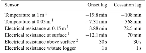
Temperature at 1 m1 −19.8 min −108 min Temperature at 0.05 m1 −7.31 min −568 min Electrical resistance at 0.15 m1 3.88 min 72.5 min Electrical resistance at surface1 −12.1 min 70 min Electrical resistance above surface2 30 s 30 s Electrical resistance w/state logger 1 s 1 s

1_{Blasch et al., 2002} 2_{Goulsbra et al., 2009}

flow events, rather than discharge, is a possibility in channels with minimal erosion and debris as long as the instrument is calibrated often in the field to avoid changes in bed height resulting in false-positives and false-negatives.

2.1.5 Floats

Generally, floats are used within stilling wells to measure the stage in the channel (Gupta, 2001). The complexity of setting up stilling wells makes them unsuitable for instances where a high spatial resolution is being sought. Also, stilling wells are not ideal for measuring ephemeral streamflow due to the potential decoupling of ground water and surface water (i.e. some ephemeral streams are likely responding more to sur-face and near sursur-face runoff inputs rather than ground water). However, the use of a float directly in an ephemeral stream has the potential to measure the stage.

Floats can be used as a measurement device in ephemeral streams to measure the maximum height reached in the chan-nel and whether flow was present during a period of time. By attaching a float to an upright with a toothed configuration that only allows upward movement, the float would move up during times of flow and hold its position unless flow reached a higher level. This method would work in sensing when wa-ter was present in a stream and the maximum height reached, however, it would be limited by the need for direct observa-tion and recording of float heights. The relatively low cost of this method would allow a great spatial resolution, however, the physical limitations would minimize its temporal resolu-tion. Using a series of sensors to detect where the float is on the upright could however improve the temporal scale and provide data on water height.

While the preceding methods of observation could be adapted to monitoring stream network extent, attempts have been made to create observation equipment specifically for the measurement of ephemeral streamflow.

2.2 Specific monitoring techniques for ephemeral streams

The advent of relatively inexpensive electronics in the 1990s allowed for new, more automated, methods of flow detection

to be created. Lower costs meant that a greater spatial res-olution could be obtained, while the automation meant that the temporal resolutions attainable were potentially finer than could be achieved through direct observation techniques. 2.2.1 Temperature sensors

Temperature sensors buried beneath the channel bed showed a marked difference in temperature when water was present in the stream compared to when the channel was empty (Con-stantz et al., 2001). The ability to distinguish the presence of water allowed the researchers to infer when there was water in the channel and when it was dry. Using temperature as a surrogate measure for the presence of water in the chan-nel makes this method less robust as it is prone to error from sudden variations in temperature, such as when a cold front passes. The data were difficult to analyze as the tempera-ture signal would ramp up and ramp down, leaving the ana-lyst to decide at what point to consider it streamflow and at what point to consider flow to have ceased (Constantz et al., 2001). Nonetheless, the lower costs of these devices allowed for greater spatial resolution of observations, while automa-tion meant that temporal resoluautoma-tion was finer than direct ob-servation.

2.2.2 Electric resistance sensors

1012 R. Bhamjee and J. B. Lindsay: Ephemeral stream sensor design using state loggers

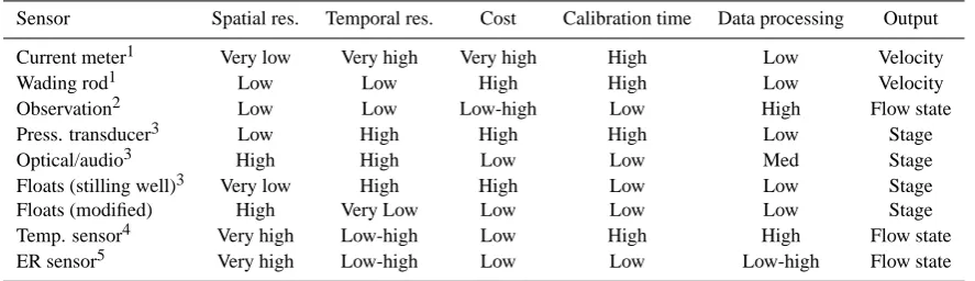
Table 2. Comparison of monitoring techniques

Sensor Spatial res. Temporal res. Cost Calibration time Data processing Output

Current meter1 Very low Very high Very high High Low Velocity

Wading rod1 Low Low High High Low Velocity

Observation2 Low Low Low-high Low High Flow state

Press. transducer3 Low High High High Low Stage

Optical/audio3 High High Low Low Med Stage

Floats (stilling well)3 Very low High High Low Low Stage

Floats (modified) High Very Low Low Low Low Stage

Temp. sensor4 Very high Low-high Low High High Flow state

ER sensor5 Very high Low-high Low Low Low-high Flow state

1_{Based on (Wahl et al., 1995)}2_{(Day, 1978; Morgan, 1972)}3_{(Gupta, 2001)}4_{(Constantz et al., 2001; Blasch et al., 2004)}5 _{(Blasch et al., 2002; Adams et al., 2006;} Goulsbra et al., 2009)

A summary of the strengths and weaknesses of the preced-ing monitorpreced-ing methods can be seen in Table 2 where spatial and temporal resolution are ideally maximized, while cost, calibration time and data processing time are minimized. Us-ing previous monitorUs-ing methods, this paper will explore the modification and enhancement of the ER sensor design to better measure changes in stream network extent.

3 Sensor design

The sensor was designed to suit the environment typically found in the predominantly agricultural catchments in South-ern Ontario. Conditions in Southern Ontario headwater streams include diverse soil types and a range of land covers. Local headwater channels frequently experience high sedi-ment transport and deposition and possess substantial vege-tative debris because of the surrounding land-cover which is typically a mixture of agriculture and forest. Another con-sideration is that with many small animals utilizing the dry channels, there is potential for the sensors to be destroyed by trampling or entanglement with the wires.

The sensor is made up of two distinct parts that were con-sidered independently to meet a set of criteria. The sensor head is the part of the sensor which contains the electrodes and is located in the channel while the logger is a dedicated unit designed to measure and record the responses of the sen-sor heads.

3.1 Sensor

Several environmental factors were considered during the sensor design. Southern Ontario agricultural basins, where the sensors were to be deployed, are made up clayey and sandy soils which are prone to erosion. As such, considera-tion for how the sensors respond to high sediment transport is important. Along the same lines, many channels have debris which is carried downstream when flow occurs. Thus, the sensor head needed to be designed such that the chances of it

being covered in sediment, destroyed by debris in the chan-nels or trampled by local wildlife was minimized. The size of the sensor heads was also an important consideration since the set up and take down of the network would mean trans-porting them through various terrain types. For this study, a balance between building a small, lightweight sensor and one which could withstand the rigors of the environment needed to be struck. To ensure that these two main criteria were met, various sensor heads were tested in the lab.

A variety of sensor head designs were lab tested in a river tray containing sediment with an average grain size of 0.3 µm. Flow was initiated from the channel head, flowing downstream. While this is not always how channels initiate, it is representative of the channel when flow is occurring. For each tested sensor head, the slope of the tray was set to 15, 10 and∼0 degrees to represent various rates of flow as well as various rates of sediment mobilization. Each sensor head was tested at three locations within the river tray (top, middle and bottom) for a minimum of thirty minutes to ensure that sediment transport results were consistent and comparable between sensor heads. As well, each sensor head tested was oriented in the ideal position, parallel to flow, as well as at a 45 degree angle to the direction of flow. Doing so ensured that the design would not fail in the event that the direction of flow in the channel was not as expected during set up. Each sensor head was also set up in a “clean” state, sitting above the bed as they would be set up in the field, as well as starting them off buried slightly under the bed to simulate the result of a sensor being covered by sediment. Refinements were made on sensor heads that showed promise until a final design was chosen.

R. Bhamjee and J. B. Lindsay: Ephemeral stream sensor design using state loggers 1013

Bhamjee & Lindsay: Ephemeral stream sensor design using state loggers 11

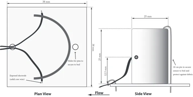
Holes for pins to secure to bed

Exposed electrode (solid core wire)

38 mm

38 mm

10 cm pin to secure sensor to bed and protect against debris

25 mm

25 mm

Plan View Flow Side View

12.5 mm

Fig. 1.Electronic resistance (ER) sensor schematic

Fig. 1. Electronic resistance (ER) sensor schematic.

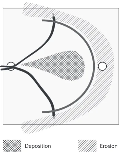
cut to 38×38 mm squares and attached using the same ma-rine glue used to seal the holes in the logger housing. The design was chosen over others due to its simplicity, consist-ing of only two parts, the cost per sensor (<$0.50 per sensor head) as well as its ability to prevent sediment settling on the electrodes. Unlike the design used by Goulsbra et al. (2009), which had the water run through a container using screens to keep out sediment, this design places the electrodes on the outside and avoids the chance of the screens being blocked by sediment. This “open” design means that care needs to be taken to ensure that sediment and other debris do not settle on the electrodes, potentially causing a false-positive (i.e. recording flow when no flow exists). The design miti-gates this by placing the electrodes in the areas where ero-sion around the sensor were shown to occur (Fig. 2). The curved design of the sensor head created an area of higher relative pressure which ensured the sediment did not build up around the electrodes as well as allowing for debris in the channel (e.g. leaves, sticks, etc.) to be deflected away from electrodes rather than being caught up on the front surface. Elevating the electrodes above the baseplate minimized the chance of sediment building up around them as well as en-suring that a signal was not present when water was stagnant (i.e. standing water) on the baseplate prior to it evaporating. By placing the electrodes on either side of the sensor head, the chance of this occurring was further avoided as was the chance that the wires would contact each other (i.e. short cir-cuit). While the sensor head design is an important consider-ation for detecting flow, the choice in data logger also has an impact on how that flow is recorded and interpreted. 3.2 Logger

Since measuring ephemeral stream flow ultimately involves identifying periods of flow and no-flow, there is no advan-tage to recording the specific electrical conductivity coming from the sensor head such as in the modified temperature

logger found in Goulsbra et al. (2009). Rather than record-ing the electrical resistance of the water, which is not needed to determine flow, state loggers were chosen. State loggers have internal resistance thresholds which are interpreted as being an open or closed circuit, that in the case of ephemeral flow monitoring can be inferred as no-flow and flow states respectively. State loggers record a value only when there is a change in the information coming from the sensor. By con-trast, interval loggers will record a value at a predetermined interval, regardless of whether a change has occurred. This monitoring strategy leads to a reduced memory capacity in the loggers when a short interval is used or the trade off of a longer measurement interval (i.e. lower temporal resolution) which is not ideal as stream network expansion is likely to be rapid after intense rainfall events in some catchments. For monitoring ephemeral stream flow timing and duration, event logging is not suitable, as there is concern about both the start and end of flow events. Measurement of ephemeral stream-flow timing and duration up to this point have used interval loggers at the expense of temporal resolution.

1014 R. Bhamjee and J. B. Lindsay: Ephemeral stream sensor design using state loggers 12 Bhamjee & Lindsay: Ephemeral stream sensor design using state loggers

Deposition Erosion

Fig. 2.Schematic of typical erosional and depositional areas around the sensor head under lab conditions.

Fig. 2. Schematic of typical erosional and depositional areas around

the sensor head under lab conditions.

The chosen data logger for this study was the Onset HOBO U-11 state logger. The U-11 includes three state logging in-puts as well as one event input (not used) which allowed for a reduced cost in data loggers compared to previous studies, where each sensor head had a dedicated logger. This reduced per-sensor cost meant that a greater spatial resolution could be achieved at a lower cost. The U-11 logger has a temporal resolution of 1 s, a far higher resolution than the phenomenon being measured, which in combination with the statelogging meant that it had the ability to drastically increase the tem-poral scale of ephemeral flow data compared to previous de-signs where logger memory was a limiting factor for tempo-ral resolution.

To test how the U-11 response time compared to previ-ous designs, notably the ER sensors used in Goulsbra et al. (2009), the electrodes were placed into a pan of water to de-termine the lag times for recording the onset and cessation of flow. Table 3 shows the lag times for the prominent sen-sor designs used in the literature. Lag times with negative numbers denote where the sensor recorded a false-positive (i.e. the presence of water in the channel, when there was no water present). This is especially an issue with the sensors that were located beneath the surface as they recorded satu-rated soil as being flow events, thus making them less suited to consistently being able to compare ephemeral streamflow at different sites. With sensors raised above the surface, the lag time is determined by the interval which the logger can record data as well as the time it takes for the water to reach the height of the electrodes. The example in Goulsbra et al.

Table 3. Lag times for sensor designs

Sensor Onset lag Cessation lag

Temperature at 1 m1 −19.8 min −108 min Temperature at 0.05 m1 −7.31 min −568 min Electrical resistance at 0.15 m1 3.88 min 72.5 min Electrical resistance at surface1 −12.1 min 70 min Electrical resistance above surface2 30 s 30 s Electrical resistance w/state logger 1 s 1 s

1_{Blasch et al., 2002}2_{Goulsbra et al., 2009}

(2009) used a 30 s interval as it allowed for the best trade off between temporal resolution and the logger memory avail-able. Since the U-11 loggers check for a change of state every one second, this allows for a very fine temporal res-olution, with minimal lag and unlike with an interval logger, the state logger minimizes the trade off.

Since the Hobo U-11 loggers were not designed for out-door use, logger housings were built using waterproof, seal-able storage containers. To accommodate the logger’s data input cables, holes were drilled in the side of the housing, allowing just enough room to insert the cables. The use of a marine glue to seal the holes allowed for a reliable water-proof seal and since the glue is able to dry in wet conditions it allowed for the repair of logger housings in the field regard-less of the weather, rather than taking a logger offline until it could be redeployed. Finally, both the logger and the sensor were connected to create a field deployable unit.

3.3 Field-ready sensor

R. Bhamjee and J. B. Lindsay: Ephemeral stream sensor design using state loggers 1015

Bhamjee & Lindsay: Ephemeral stream sensor design using state loggers 13

Fig. 3.RARE study sites

Fig. 4.Rondeau Bay study sites

Fig. 3. RARE study sites.

the sensor head and one behind. The placement of the front peg, other than acting as an anchor, also helped to protect the sensor from larger debris

4 Field set-up and siting considerations

While extensive lab testing was completed, the sensors needed to be tested in the field to truly determine their us-ability. Unlike the controlled environment of the lab, the individual constraints on each sensor head were less struc-tured, but tried to account for as many scenarios as the study sites would allow.

4.1 Study sites

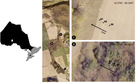
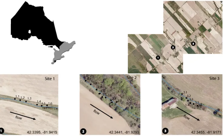
Field testing occurred at the RARE Charitable Reserve (Fig. 3), which is a part of the Grand River watershed in Ontario, Canada as well as in the Rondeau basin (Fig. 4) in southwestern Ontario .

The RARE Charitable Reserve is mainly composed of ac-tive and fallow agricultural fields, forest and low-lying boggy forested areas. The wide variety of land-use/land cover types and sediment types meant the sensors could be tested in many of the characteristic types of landscapes to be found in Southern Ontario. Testing on the site was around Cruickston Creek, which is a tributary of the Grand River. Ephemeral channel widths available on at the site ranged from 10 cm to over 30 cm with degrees of slope similar to those used in the lab tests. Available channel depths at the study site ranged from 5 cm to 15 cm. Vegetation at RARE included mixed de-ciduous and coniferous forests, fallow fields with tall grasses and plants (e.g. thistle), winter wheat and ground cover type plants in the boggy areas (e.g. skunk cabbage – Symplocar-pus foetidus).

The Rondeau basin is located in southwestern Ontario and drains into Lake Erie through a series of deep headwater gul-lies, which originate on a plateau in the north, and larger

streams further downstream in the channel network. Many of the gullies in the area experience emphemeral flow. There are many problems with sediment and nutrient transport within the watershed, especially off of agricultural fields, that have led to severe eutrophication of Rondeau Bay (Lam-bert, 1997). Frequent in-filling of channels that cross through fields is done to reduce the amount of sediment loss from agricultural fields. Likewise, gullies adjacent to fields tend to be deepened to promote quick removal of water off of tile-drained fields. As a result of steep gullies and anthropogenic modification, the basin has many ephemeral channels in the headlands that run through different types of land-uses/land covers as well as vary in size and depth. The channel widths used for the study ranged from 15 cm to over 200 cm while the depths used were between 10 cm to over 200 cm. Vege-tation in the basin is mainly agricultural, with wheat, corn and soybeans being the predominant crop types, however, the catchment also includes deciduous forests and hedgerows separating fields. Unlike the RARE site, the sites in Rondeau did not feed into a single, perennial stream nearby, but rather had a greater spatial distribution and less connectivity via a common stream network.

4.2 Network installation

Five sets of loggers, each set containing three sensor heads, were installed within headwater channels of the RARE site to capture each type of land-use in the area. In Rondeau, seven set of loggers, also with three sensor heads were in-stalled within ephemeral channels at the study sites within the basin. Within the channel, sensors were placed in the thalweg to ensure they were in the path of the flow which was not always in the centre of the channel. Each sensor was placed on a local riffle rather than in a pool to minimize the possibility that sensors could be situated in standing water (i.e. puddles within pools) for extended periods. In doing so, the responsiveness of the sensors to actual flow periods was increased. To reduce the likelihood of animals interfering with the wire cables connecting the sensors to the loggers, cables were buried or placed under rocks or logs.

Data loggers were situated near channel banks closest to the middle sensor and were secured in place to prevent move-ment. The loggers allowed for about 1.5 months of data logging depending on the number of events. Whenever data from the loggers were downloaded, sensors were checked to ensure they were not covered in sediment and if a channel cross-section had changed significantly between field visits, sensors were re-situated within the thalweg.

1016 R. Bhamjee and J. B. Lindsay: Ephemeral stream sensor design using state loggers Bhamjee & Lindsay: Ephemeral stream sensor design using state loggers 13

Fig. 3.RARE study sites

Fig. 4.Rondeau Bay study sites Fig. 4. Rondeau Bay study sites.

5 Data processing

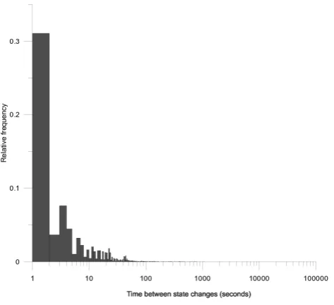
Figure 5 shows a sample data set both in raw and post-processed form. In the raw data set, around the time of a change of state (i.e. from flow to no-flow or vise versa), the state change is associated with numerous and frequent records that can be considered noise. This noise was also ob-served in lab testing, especially when the channel slope was low. It is believed that this observed noise in the data, around times of changes in state, occurs when the water level is very near the height of the electrodes (1.5 cm). Ripples in the wa-ter surface due to turbulence or wind around the critical level of the electrodes are responsible for these short time-scale changes of state. Figure 6 presents a frequency distribution of the time between state changes in the data set. It is ap-parent that there is a rapid decrease in the frequency of state changes as events become longer (i.e. actual drying and wet-ting events).

Noise was removed from the dataset where these changes of state occurred at frequencies greater than 30 s. A 30 s in-terval was selected due to fact that it was unlikely that a chan-nel could fill and empty in less than 30 s. To remove noise, the first wet state recorded was selected for the start of a flow event, while the last dry state in the data was selected. It can be assumed that the first wet state is when the water has reached the height of the electrodes, while the subsequent dry and wet data points are the water level fluctuating above and below the electrodes. The last dry state signifies where the water is no longer in flux over the electrodes, meaning that there was either no water in the channel, or very little water which is either stagnant or reducing in depth. Noise events occurred for periods as short as two seconds (two state

14 Bhamjee & Lindsay: Ephemeral stream sensor design using state loggers

a)

b) No Flow

Flow

No Flow Flow

Fig. 5.Raw data(a)and post-processed data(b)with the noise removed for one sensor head.

Fig. 5. Raw data (a) and post-processed data (b) with the noise

removed for one sensor head.

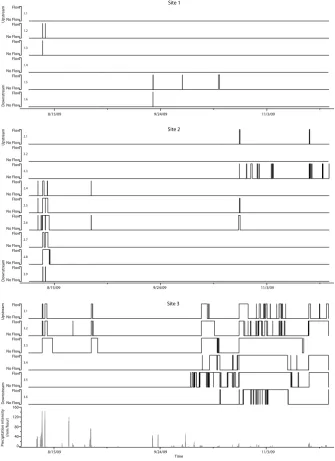
changes) and as long as about one hour (3600 state changes). The former occured during the onset of flow, while the longer noise events were during cessation periods. This can be com-pared to a typical hydrograph, where the onset of flow oc-curs quickly, but the cessation of flow ococ-curs gradually. By removing noise from the data, individual flow events were more easily highlighted and better represented the situation in the channel at the time of the event. The flow state data from Rondeau with the noise removed can be seen in Fig. 7 along with precipitation intensity for the monitoring period.

6 Network expansion

R. Bhamjee and J. B. Lindsay: Ephemeral stream sensor design using state loggers 1017

Bhamjee & Lindsay: Ephemeral stream sensor design using state loggers 15

Fig. 6.Histogram showing relative frequency of sensor response times (i.e. off to on and vise versa)

Fig. 6. Histogram showing relative frequency of sensor response

times (i.e. off to on and vise versa).

network expansion which were observed in the data (Fig. 8). Headward expansion is the growth of the flowing channel from a downstream position towards the channel head as a result of soil saturation. Downstream expansion is the move-ment of water from the headland areas which fills the channel from its upper reaches initially and flows downstream until it meets the perennial channel. Downstream expansion is gen-erally caused by the inability for precipitation to infiltrate the surface either due to a high intensity of rainfall and/or low infiltration capacity (Ward and Robinson, 2000). The coa-lescence model of expansion results when small pools form along the length of the channel until they eventually connect to form a flowing stream. This model of expansion results from the saturation and in-filling of local low spots that even-tually expand outward as they fill. There are also instances where a cross-section within a channel may respond, but the stream does not expand. In this case, these single sensor re-sponses can be inferred to be incomplete coalescence.

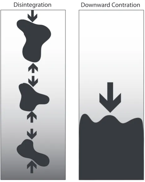
While three models of expansion exist, there are only two models of contraction: downstream contraction and disinte-gration (Fig. 9). Downstream contraction occurs as each sen-sor turns off starting at the channel head, moving downstream (i.e. the stream network dries out from the channel heads down toward the perennial stream). Disintegration, similar to coalescence occurs when flow ceases and local pools re-main and drain or lose water through evaporation. Instances where it appears the stream is contracting headward are bet-ter described by the disintegration model since continuous flow stops as soon as the bottom-most sensor turns off. Ex-pansion and contraction responses from the study sites can be seen in Tables 4 and 5 as well as the average percent of occurrence for all the sites.

Table 4. Occurrence of each model of expansion as a percent of all

events.

Stream network expansion

Downstream Upward Coalescence Site expansion expansion Complete Incomplete

1 10 15 35 40

2 5.88 5.88 23.53 64.71

3 0 0 40 60

All sites 7.14 9.52 30.95 52.38

Table 5. Occurrence of each model of contraction as a percent of

all events.

Stream network contraction

Downstream Disintegration

Site contraction Complete Incomplete

1 20 40 40

2 0 35.41 64.71

3 0 40 60

All sites 9.52 38.09 52.38

Incomplete coalescence was the most common occurrence at all three sites, however, these were not showing expansion nor contraction. Coalescence and disintegration were by far the prevalent expansion and contraction models found across all the sites. The related models of coalescence and disinte-gration accounted for nearly 85% of all network expansion and contraction events. On a site-to-site basis, expansion and contraction models were found to vary over the course of the monitoring period. As stated earlier, the model of expan-sion does not always yield the corresponding model of con-traction. For instance, site 1 had 10% of expansion events where downstream expansion occurred and 20% of events where downstream contraction occurred. Site 3 was by far the least varied site never showing expansion nor contraction by upward expansion or downstream expansion or contrac-tion. Site 2 was also quite consistent with just over 12% of expansion events being downstream expansion or upward ex-pansion models and all contraction events being disintegra-tion. The way a channel responds is presumably controlled by the characteristics of both the channel itself, as well as processes of water delivery that are ongoing within the adja-cent hillslopes.

1018 ₁₆ R. Bhamjee and J. B. Lindsay: Ephemeral stream sensor design using state loggers_{Bhamjee & Lindsay: Ephemeral stream sensor design using state loggers}

11/3/09 Time

9/24/09 8/15/09

Pr

ecipita

tion in

tensit

y

(mm/hour)

D

ownstr

eam

Upstr

eam

D

ownstr

eam

Upstr

eam

D

ownstr

eam

Upstr

eam

11/3/09 9/24/09

8/15/09

11/3/09 9/24/09

8/15/09

Site 1

Site 2

Site 3

Flow

No Flow Flow

No Flow Flow

No Flow Flow

No Flow Flow

No Flow Flow

No Flow Flow

No Flow Flow

No Flow Flow

No Flow Flow

No Flow Flow

No Flow Flow

No Flow Flow

No Flow Flow

No Flow Flow

No Flow Flow

No Flow Flow

No Flow Flow

No Flow Flow

No Flow Flow

No Flow Flow

No Flow 1.1

1.2

1.3

1.4

1.5

1.6

2.1

2.2

2.3

2.4

2.5

2.6

2.7

2.8

2.9

3.1

3.2

3.3

3.4

3.5

3.6

160

120

80

40

0

Fig. 7.Final flow data from field with noise removed Fig. 7. Final flow data from field with noise removed.

topography, land use/land cover, and anthropogenic activ-ities (e.g. tile drains). In-channel characteristics that are relevant to how the channel delivers water downstream in-clude, cross-sectional channel geometry, longitudinal pro-file (i.e. slope and pool characteristics), roughness (includ-ing the abundance and type of vegetation) and modification of the channel (e.g. straightening, widening, etc.). The com-bination of these characteristics should affect the manner in which a stream expands and contracts. How a channel ex-pands does not inherently dictate how the channel will con-tract, nor does the prevalent manner by which the channel expands or contracts guarantee that it will respond the same

way under all conditions. However, under similar initial con-ditions, channels are expected to respond in a similar manner.

7 Discussion

R. Bhamjee and J. B. Lindsay: Ephemeral stream sensor design using state loggers 1019

Bhamjee & Lindsay: Ephemeral stream sensor design using state loggers

17

n o i s n a p x e d r a w d a e H n o i s n a p x e m a e r t s n w o D Coalescence

Fig. 8.

Models of stream network expansion. Coalescence: the

formation of individual pools which join to create a flowing

net-work; Downstream expansion: movement of water from upstream

to downstream; Headward expansion: movement of the channel

head upstream.

Fig. 8. Models of stream network expansion. Coalescence: the

formation of individual pools which join to create a flowing net-work; Downstream expansion: movement of water from upstream to downstream; Headward expansion: movement of the channel head upstream.

The main limitation of the ER sensor design is that it is only measuring wet and dry states, rather than flow or no-flow states. While it can be assumed that in many situations, a wet state will be a flowing state due to the fact that the sensors were places on riffles, it cannot be guaranteed. This has been a limitation of all previous approaches as well, in-cluding methods based on ambient bed temperature and ER. Lab experiments have been conducted previously to explore the possibility of measuring flow and no-flow timing directly. These sensor designs were seriously hindered by their lack of robustness in the presence of sediment transport.

While attaching three sensors to a single logger reduced the overall cost of the sensor network, allowing for greater spatial resolution of measurements, logger memory capac-ity was filled more quickly than it would have if each sensor had a dedicated logger. However, since the logger recorded changes of state, the memory lasted much longer than pre-vious sensor designs where each sensor had its own logger. Another trade-off with having three inputs into one logger was that if a logger failed, three points of measurement along a stream would be lost. While there is no guaranteed way to ensure a logger will not fail for a variety of reasons, frequent monitoring of the sites reduces the chance of this happen-ing. Noise in the data was another factor which needed to be accounted for in the sensor network design and data post-processing.

While compared to previous attempts, using ER sensors (Goulsbra et al., 2009; Adams et al., 2006), or the bed-temperature method (Blasch et al., 2004) the use of a state logger has allowed for a drastic reduction in post-processing

18 Bhamjee & Lindsay: Ephemeral stream sensor design using state loggers

Disintegration Downward Contration

Fig. 9.Models of stream network contraction. Disintegration: the

breaking up of a flowing reach into drying pools. Downward con-traction: movement of the channel head downstream.

Fig. 9. Models of stream network contraction. Disintegration: the

breaking up of a flowing reach into drying pools. Downward con-traction: movement of the channel head downstream.

of data while also increasing the temporal resolution because there is no need to determine a sensor-specific threshold in ER. Noise in the data was due to the high temporal reso-lution of the loggers recording ripples forming on the sur-face of channel at the level of the electrodes. Site condi-tions, mainly saturation of soil, affected how quickly streams began to flow. Some channels responded very quickly and showed no noise, while others displayed a slower rise, thus leading to rippling and in turn, noise. While the sensitivity of the current design allows for a very fine temporal resolution which shows the instantaneous rise and fall of the water level above and below the electrodes, a decrease in the sensitivity of the sensor head would allow for cleaner data set for study-ing longer time frames without the need for post-processstudy-ing work.

1020 R. Bhamjee and J. B. Lindsay: Ephemeral stream sensor design using state loggers worked as expected under the tested flow conditions. The

sensors performed well in the field, with the main draw-back being that if they were not correctly placed in a chan-nel cross-section, it was possible that low flows were missed as they diverted around the sensor head. Along these same lines, the height of the electrodes meant that any flow in the channel under 12.5 mm would not have been recorded. How-ever, as coalescence was the dominant model of expansion, measuring these extremely low water levels would not have showed real flow, but rather puddling at an earlier stage. This also has the potential to add significant amounts of noise as described previously. Noise as a result of debris contacting the electrodes was not noticed at any of the sites. The sensor design has allowed for the study of ephemeral streamflow duration and timing in a more quantitative manner.

While the models of expansion presented in this paper are applicable to many landscapes, the scale at which the study is focusing must be considered. At one scale, part of a stream network may appear to expand by way of upward expansion, but when observing the network at another scale, coalescence may be the model which dominates expansion. Accuracy in determining how the entire network expands and contracts hinges on being able to monitor the entire network at fine spatial resolution. Utilizing an inexpensive sensor such as the one presented in this paper will allow for this fine spatial res-olution to be determined. Temporal scale is also an important consideration as some channels will flow quickly and having a longer interval will mean that the expansion model could be misrepresented. However, networks will most likely dis-play various models of expansion and contraction depending on the characteristics of each channel and it’s surrounding slopes as well as the initial conditions prior to flow.

The ability to deploy the sensors for long periods of time, in a variety of physical environments, has allowed for an improvement in the ability to study the expansion and con-traction of stream networks. The cost and ease of setup and maintenance mean that the sensors can be setup at a variety of locations within different regions. This greatly improves the ability to quantitatively compare the behaviour of channels to each other. In doing so, characteristics of each channel can be compared to determine the controls on expansion and contraction as well as observe the manner in which stream networks expand and contract. Knowing this allows for a better understanding of the role headland areas play in the dynamics of the entire watershed. In predominantly agricul-tural basins, such as Rondeau, this is especially important as the modification and location of these streams has a great affect on downstream water quality and quantity.

8 Conclusions

This study describes a novel sensor and monitoring network design for measuring stream flow timing and duration in ephemeral channels in Southern Ontario. The following con-clusions can be drawn from this work:

1. State logging lessened the amount of noise in the data and the subjectivity in the interpretation of events when compared to previous attempts at measuring ephemeral streamflow using electrical resistance, while also in-creasing the responsiveness to flow events and eliminat-ing the need for per-sensor calibration.

2. Spatial and temporal resolution was increased through the use of the state logger. Three inputs allowed for a greater spatial scale due to the lower relative cost and since only changes in state were recorded, temporal res-olution was increased relative to previous sensor de-signs as the logger checked for a change of state every second.

3. Generic models of flow can be used to describe the ex-pansion and contraction of stream networks to study the dynamic of ephemeral steamflow at different scales. 4. Monitoring ephemeral stream duration and timing is

needed to understand the dynamics of the flowing stream network. In doing so, the understanding of the migration and fate of pollutants can be enhanced.

Supplementary material related to this article is available online at:

http://www.hydrol-earth-syst-sci.net/15/1009/2011/ hess-15-1009-2011-supplement.zip.

Acknowledgements. Thank you to Stewart Sweeny and Doug

Aspinal at OMAFRA and Greg Dunn at MNR for their help with finding study sites in Rondeau and Peter Kelly for his help at RARE.

Edited by: N. Basu

References

Adams, E. A., Monroe, S. A., Springer, A. E., Blasch, K. W., and Bills, D. J.: Electrical resistance sensors record spring flow tim-ing, grand canyon, arizona, Ground Water, 44(5), 630–641, 2006. Arnell, N.: Hydrology and global environmental change, Pearson

Education, 20002.

Bardossy, A. and Lehmann, W.: Spatial distribution of soil moisture in a small catchment. part 1: geostatistical analysis, J. Hydrol., 206(1–2), 1–15, 1998.

R. Bhamjee and J. B. Lindsay: Ephemeral stream sensor design using state loggers 1021

Blasch, K. W., Ferre, T. P. A., Christensen, A. H., and Hoffmann, J. P.: New field method to determine streamflow timing us-ing electrical resistance sensors, Vadose Zone J, 1(2), 289–299, 2002.

Blasch, K. W., Ferre, T. P. A., and Hoffmann, J. P.: A statistical tech-nique for interpreting streamflow timing using streambed sedi-ment thermographs, Vadose Zone J, 3(3), 936–946, 2004. Blyth, K. and Rodda, J. C.: A stream length study, Water Resour.

Res., 9(5), 1454–1461, 1973.

Burt, T. and Butcher, D.: On the generation of delayed peaks in stream discharge, J. Hydrol., 78(3–4), 361–378, 1985.

Constantz, J., Stonestorm, D., Stewart, A. E., Niswonger, R., and Smith, T. R.: Analysis of streambed temperatures in ephemeral channels to determine streamflow frequency and duration, Water Resour. Res., 37(2), 317–328, 2001.

Day, D. G.: Drainage density changes during rainfall, Earth Surf. Proc., 3(3), 319–326, 1978.

Day, D. G.: Lithologic controls of drainage density: A study of six small rural catchments in New England, N.S.W, CATENA, 7(4), 339–351, 1980.

Dunne, T. and Black, R. D.: Partial area contributions to storm runoff in a small New England watershed, Water Resour. Res., 1970.

Ensign, S. and Doyle, M.: Nutrient spiraling in streams and river networks. J. Geophys. Res., 111(G4), G04009, doi:10.1029/2005JG000114, 2006.

Gomi, T., Sidle, R., and Richardson, J.: Understanding processes and downstream linkages of headwater systems, BioScience, 52(10), 905–916, 2002.

Goulsbra, C., Lindsay, J., and Evans, M.: A new approach to the application of electrical resistance sensors to measuring the onset of ephemeral streamflow in wetland environments. Water Resour. Res., 45(9), W09501, doi:10.1029/2009WR007789, 2009. Gregory, K. and Ovenden, J.: Drainage network volumes and

pre-cipitation in Britain, Transactions of the Institute of British Ge-ographers, 4(1), 1–11, 1979.

Gregory, K. and Walling, D.: The variation of drainage density within a catchment, Bull. Int. Ass. Sci. Hydrol., 13(2), 61–68, 1968.

Gupta, R.: Hydrology and hydraulic systems, Waveland Press, 2001.

Labbe, T. and Fausch, K.: Dynamics of intermittent stream habitat regulate persistence of a threatened fish at multiple scales, Eco-logical Applications, 10(6), 1774–1791, 2000.

Lambert, L.: Technical report no. 15: degredation of aesthetics, Lake Erie Lakewide Management Plan (LaMP) Technical Report Series, 1997.

McClain, M. E., Boyer, E. W., Dent, C. L., Gergel, S. E., Grimm, N. B., Groffman, P. M., Hart, S. C., Harvey, J. W., Johnston, C. A., Mayorga, E., McDowell, W. H., and Pinay, G.: Biogeo-chemical hot spots and hot moments at the interface of terrestrial and aquatic ecosystems, Ecosystems, 6(4), 301–312, 2003. Meyer, J., Strayer, D., Wallace, J., Eggert, S., Helfman, G., and

Leonard, N.: The contribution of headwater streams to biodiver-sity in river networks, J. Am. Water Resour. As., 43(1), 86–103, 2007.

Meyer, J. and Wallace, J.: Lost linkages and lotic ecology: rediscov-ering small streams. 295–317, Ecology: achievement and chal-lenge. Blackwell Science, Oxford, UK, 406, 2001.

Morgan, R. P. C.: Observations on factors affecting the behaviour of a first-order stream, Transactions of the Institute of British Geographers, 171–185, 1972.

Mulholland, P., Tank, J., Sanzone, D., Wollheim, W., Peterson, B., Webster, J., and Meyer, J.: Nitrogen cycling in a forest stream determined by a 15N tracer addition, Ecological Monographs, 70(3), 471–493, 2000.

Peterson, B., Wollheim, W., Mulholland, P., Webster, J., Meyer, J., Tank, J., Marti, E., Bowden, W., Valett, H., Hershey, A., McDowell, W. H., Dodds, W. K., Hamilton, S. K., Gre-gory, S., Morrall, D. D.: Control of nitrogen export from watersheds by headwater streams. Science, 292(5514), 86–90, doi:10.1126/science.1056874, 2001.

Poff, N., Allan, J., Bain, M., Karr, J., Prestegaard, K., Richter, B., Sparks, R., and Stromberg, J.: The natural flow regime, Bio-Science, 47(11), 769–784, 1997.

Quinn, P., Beven, K., Chevallier, P., and Planchon, O.: The predic-tion of hillslope flow paths for distributed hydrological modelling using digital terrain models, Hydrol. Process., 5(1), 59–79, 1991. Wahl, K. L., Thomas, W. O., and Hirsch, R. M.: Stream-gaging

program of the US Geological Survey, 1995.