https://doi.org/10.5194/hess-22-4583-2018 © Author(s) 2018. This work is distributed under the Creative Commons Attribution 4.0 License.
Technical note: Pitfalls in using log-transformed flows
within the KGE criterion
Léonard Santos, Guillaume Thirel, and Charles Perrin
Irstea, HYCAR Research Unit, 1 rue Pierre-Gilles de Gennes, 92160 Antony, France
Correspondence:Léonard Santos ([email protected])
Received: 29 May 2018 – Discussion started: 8 June 2018
Revised: 22 August 2018 – Accepted: 23 August 2018 – Published: 30 August 2018
Abstract.Log-transformed discharge is often used to
calcu-late performance criteria to better focus on low flows. This prior transformation limits the heteroscedasticity of model residuals and was largely applied in criteria based on squared residuals, like the Nash–Sutcliffe efficiency (NSE). In the re-cent years, NSE has been shown to have mathematical limi-tations and the Kling–Gupta efficiency (KGE) was proposed as an alternative to provide more balance between the ex-pected qualities of a model (namely representing the water balance, flow variability and correlation). As in the case of NSE, several authors used the KGE criterion (or its improved version KGE0) with a prior logarithmic transformation on flows. However, we show that the use of this transformation is not adapted to the case of the KGE (or KGE0) criterion and may lead to several numerical issues, potentially resulting in a biased evaluation of model performance. We present the theoretical underpinning aspects of these issues and concrete modelling examples, showing that KGE0 computed on log-transformed flows should be avoided. Alternatives are dis-cussed.
1 Introduction
In the context of rainfall–runoff modelling, evaluating the quality of the models’ outputs is essential. Deterministic sim-ulations are commonly evaluated using efficiency criteria such as the Nash–Sutcliffe efficiency (NSE, Nash and Sut-cliffe, 1970). The choice of the criteria obviously depends on the modeller’s objective. For example, one may wish to fo-cus on the overall water balance evaluation, or more specif-ically on the simulation of different flow ranges – typspecif-ically high, intermediate or low flows. For these different
objec-tives, given that the model residuals are generally not ho-moscedastic and often depend on the flow magnitude, one common option to focus more closely on specific flow ranges is to apply various prior transformations on the simulated and observed discharge time series to distort the range of errors, which consequently changes the relative weight of different flow ranges in the criterion. This is commonly done within the NSE criterion, which has been one of the most popu-lar criteria used in hydrological modelling in the past few decades. NSE is the distance to 1 of the ratio between the mean square error of the model and the variance of observed flows. Compared to the basic criterion computed on untrans-formed flows, a prior squared transformation on flows would put even more weight on high flows, and a logarithmic or in-verse transformation would put more weight on low flows, while a square-root transformation would have an intermedi-ate effect (Krause et al., 2005; Oudin et al., 2006; De Vos and Rientjes, 2010; Pushpalatha et al., 2012).
However, the Nash–Sutcliffe criterion was shown to have limitations. Indeed, using a decomposition of NSE based on the correlation, bias and ratio of variances, Gupta et al. (2009) clearly demonstrated that discharge variability is not correctly taken into account for the evaluation. Therefore, Gupta et al. (2009) proposed a new criterion, the Kling– Gupta efficiency (KGE), which was then improved into a modified criterion called KGE0 (Kling et al., 2012). KGE combines the previous components of NSE (correlation, bias, ratio of variances or coefficients of variation) in a more bal-anced way. It corrects the underestimation of variability and provides direct assessment of four aspects of discharge time series, namely shape, timing, water balance and variability.
flows before computing KGE, e.g. to put more weight on low flows, as done with NSE. For example, Pechlivanidis et al. (2014) applied the logarithmic transformation to use it as a benchmark for fitting a model on low flows. Seeger and Weiler (2014) used it as an objective function. Beck et al. (2016) used the untransformed and log-transformed flows in NSE,R2and KGE as an evaluation of different global mod-els, and Quesada-Montano et al. (2018) also used it as an evaluation criterion of the HBV model outputs.
In this technical note we show that the use of a logarith-mic transformation when computing KGE or KGE0, applied in a similar way to with NSE, introduces numerical flaws and should be avoided. After reviewing the mathematical formu-lation of KGE0, we expose the theoretical aspects explain-ing these flaws and illustrate them with modellexplain-ing examples. Then we suggest alternatives to circumvent this issue. The tests will be carried out using KGE0 but they are also valid for the initial KGE formulation.
2 The KGE and KGE0formulations
The KGE and KGE0criteria (Gupta et al., 2009; Kling et al., 2012, respectively denotedEKGandEKG0 in Eq. 1 and Eq. 2)
are written as a linear transformation (f :x7−→1−x) of the Euclidian distance to an ideal value (i.e. [1,1,1]) in a three-dimensional space defined by three components of the mod-elling error:
EKG=1−
q
(r−1)2+(β−1)2+(α−1)2, (1)
EKG0 =1− q
(r−1)2+(β−1)2+(γ−1)2, (2)
in which
– r, the Pearson correlation coefficient, evaluates the error in shape and timing between observed (Qo) and
simu-lated (Qs) flows: r=cov(Qo, Qs)
σ2 oσs2
, (3)
where “cov” is the covariance between observation and simulation and σ is the standard deviation, with sub-scripts “o” and “s” standing for observed and simulated, respectively.
– β, the bias term, evaluates the bias between observed and simulated flows:
β= µs
µo
, (4)
whereµ is the mean also with subscripts “o” and “s” standing for observed and simulated, respectively.
– α, the ratio between the simulated and observed stan-dard deviations, evaluates the flow variability error:
α=σs
σo
. (5)
– γ, the ratio between the simulated and observed coeffi-cients of variation (CV), also evaluates the flow vari-ability error. These coefficients of variation are used to avoid the impact of bias on the variability indica-tor (Kling et al., 2012):
γ=µoσs
σoµs
. (6)
The KGE0 values range between−∞and 1, as for NSE, and it is positively oriented.
3 Issues associated with the use of a prior logarithmic
transformation
3.1 Instability when the moments of log-transformed
flows become close to zero
Because the three termsγ,β andr are ratios, they can be-come overly sensitive to the denominator values (here µo, µs, σo or σs) if they become close to zero. In this case, a
small absolute variation in the moments’ values can tively impact the related ratio and thus produce very nega-tive KGE0 values. It is generally unlikely that values ofσo, σs,µs andµoso close to zero can be obtained to produce
numerical instability when using untransformed flows. How-ever, when a prior logarithmic transformation is applied, the values ofµlog,oorµlog,s (more rarelyσlog,oorσlog,s)
com-puted on transformed values can become equal or close to zero (because log(1)=0). The corresponding ratiosr,βorγ
would therefore become very large, leading to strongly nega-tive KGE0values. Thus a small relative difference can lead to very different conclusions. In this case, the score value does not adequately represent the qualities of the model simula-tion.
3.2 Dependence on the flow unit chosen
observed flow calculation, the conversion from cubic metres per second to litres per second gives the following:
µlog,o[L s−1] =log(1000)+µlog,o[m3s−1]. (7)
Consequently, because the conversion term becomes ad-ditive when applying the logarithmic transformation, theβ
ratio value is modified. Similarly, the γ ratio is also al-tered. Therefore, if the logarithmic transformation is used, the KGE0 (and also the KGE) is no longer a dimensionless value. This can lead to interpretation problems.
3.3 Dependence on the constant added to avoid the
zero-flow issue
When using a logarithmic (or an inverse) transformation, the case of null flows, which may exist in the case of intermittent or ephemeral streams, prevents proper calculation. To avoid this, different techniques may be set up in the case of NSE:
– The first involves discarding the zero-flow values from the series, i.e. considering them as gaps (see for example Nguyen and Dietrich, 2018). The drawback is that parts of the hydrographs become neglected, though they can bring important information on the processes at play.
– The second involves adding a small constant to all flow values (Pushpalatha et al., 2012), typically a fraction of average flow. This option is widely used and Push-palatha et al. (2012) showed that the NSE value has limited sensitivity to this constant with a logarithmic transformation as long as it is small enough compared to flow values. These authors advise a constant equal to 1/100 of the mean observed flows. But the dependence of KGE0 on this constant has not been investigated so far.
– The third involves using a Box–Cox transformation to reproduce the effects of the logarithmic transformation without the zero-flow issue (Box and Cox, 1964; Hogue et al., 2000; Vázquez et al., 2008).
4 Testing methodology
To illustrate these numerical issues and their potential im-pacts, several tests were carried out in a wide range of catch-ments, using the GR4J rainfall–runoff model (Perrin et al., 2003).
4.1 Catchment set and data
[image:3.612.310.548.63.325.2]A daily data set of 240 catchments across France (Fig. 1), set up by Ficchí et al. (2016), was used. The climate data of the SAFRAN daily reanalysis (Vidal et al., 2010) were used as input data. Precipitation and temperature were spa-tially aggregated in each catchment since the GR4J model is lumped. Potential evapotranspiration was calculated using
Figure 1.Location of the 240 flow gauging stations in France used
for the tests and their associated catchments.
a temperature-based formula (Oudin et al., 2005). Full de-tails on this data set are available in Ficchí et al. (2016). Ob-served flows were retrieved for each catchment outlet from the Banque HYDRO (http://www.hydro.eaufrance.fr/ (last access: 29 August 2018), Leleu et al., 2014). The availability of data covers the 2005–2013 period. To avoid requiring a snow model, the catchments with less than 10 % of precipi-tation falling as snow were selected.
4.2 Model and calibration
● ● ● ● ● ● ● ● ● ● ● ● ● ● ● ● ● ● ● ●●●●● ● ● ● ● ● ● ● ● ● ●●●● ● ● ● ●● ● ● ● ● ● ● ● ● ● ● ● ● ● ● ● ● ●● ● ● ● ● ●● ● ● ● ● ● ● ● ●● ● ●● ● ●● ● ● ● ● ● ● ●● ● ● ● ● ● ● ● ● ●● ● ● ● ● ● ● ● ● ● ● ● ● ● ● ● ● ● ● ● ● ● ● ● ● ● ● ●● ●●● ●● ● ● ●● ● ● ●●●●●●●●● ● ● ● ● ● ● ● ●● ● ● ● ● ● ● ● ● ● ●● ● ●● ● ● ● ● ● ● ● ● ● ● ● ● ● ●● ● ● ● ● ●●●● ● ● ● ● ● ● ● ● ● ● ● ● ● ● ● ● ● ● ●● ● ● ● ● ● ●● ● ● ● ● ● ● ● ● ● ● ● ● ● ● ●● ● ●
−2 0 2 4
−8 −6 −4 −2 0
Observations
µlog,o [m3.s−1]
KGE' on log(Q)
(a)
● ● ●
µlog,s [m3.s−1] µlog,s [m3.s−1]
−5 − −0.5 −0.5 − 0.5 0.5 − 5
● ● ● ● ● ●● ● ● ● ● ● ● ● ● ● ● ● ● ●●● ●●● ● ● ● ● ● ● ●● ● ●●●● ● ● ●● ● ● ● ● ● ● ● ●●● ● ● ● ● ● ● ●● ● ● ● ● ●● ● ● ● ● ● ● ● ●● ● ●● ● ●● ● ● ● ● ● ● ●● ● ● ● ● ●●●●●● ● ● ● ● ● ● ● ● ● ● ● ● ● ● ● ● ● ● ● ● ● ● ● ● ● ● ● ●●●●●● ● ● ●● ● ● ●●●●●●●●● ● ● ● ● ● ● ● ●●● ● ● ● ●● ● ● ● ●● ●● ●● ● ● ● ● ● ● ●● ● ● ● ●●● ● ● ● ● ●●●● ●● ● ● ● ● ● ● ● ● ● ● ● ● ● ● ● ● ●● ● ● ● ● ● ●● ● ● ● ● ● ● ● ● ● ● ● ● ● ● ●●● ●
−4 −2 0 2 4
−8 −6 −4 −2 0
Simulations
µlog,s [m3.s−1]
KGE' on log(Q)
(b)
● ● ●
µlog,o [m3.s−1] µlog,o [m3.s−1]
−5 − −0.5 −0.5 − 0.5 0.5 − 5
● ● ● ● ●●●● ●●●● ●●● ● ● ●● ●●● ●● ● ●●●●●● ●●●●●●●●●●●●●●● ●●●●● ● ●● ● ● ●●●● ●● ● ● ●● ●●● ● ● ● ● ● ● ●● ● ●●●● ●● ●● ●●●●●●●● ●●●●●●●●●● ● ●●● ● ● ● ● ●● ● ● ●●● ● ● ● ● ● ●● ●●● ● ● ●●●●●●●●●●●●●●●●●●●●●●●●●●●●●●● ●● ● ● ● ●● ●● ●●● ● ● ●● ● ●● ●●●●●●●●● ●●●● ●● ● ● ● ● ● ● ● ● ●● ● ●●● ●●●● ● ●● ● ● ●●● ● ●● ● ● ●● ●● ● ● ● ● ● ●● ● ●
−2 0 2 4
−8
−6
−4
−2
0
µlog,o [m3.s−1]
KGE' on Q
(c)
● ● ●
µlog,s [m3.s−1] µlog,s [m3.s−1]
−5 − −0.5 −0.5 − 0.5 0.5 − 5
● ● ● ●●● ●●● ●●●● ●● ● ● ●●●● ●● ●● ● ●●● ●●●●● ●●●●●●●●●● ●●●●●●●●●●● ● ●●●● ●● ● ● ● ●● ● ● ● ● ● ● ● ● ●● ● ●●●●●● ●● ● ● ●●●●●●● ●● ●●●●●● ● ● ●● ● ●● ●●●●●● ●● ●●● ● ● ●●● ●● ●●●●●●●●●●●●●● ●●●●●●●●●●●●●●●●●●●● ●● ● ● ● ●● ●●● ●●●● ● ● ● ●●●●●●●●● ●●●●●●●●● ● ●● ● ● ● ●● ● ● ●● ● ●●●● ● ●● ● ● ●● ●●● ●● ●●● ●● ● ● ● ● ● ● ●● ●
−4 −2 0 2 4
−8
−6
−4
−2
0
µlog,s [m3.s−1]
KGE' on Q
(d)
● ● ●
µlog,o [m3.s−1] µlog,o [m3.s−1]
[image:4.612.54.286.67.282.2]−5 − −0.5 −0.5 − 0.5 0.5 − 5
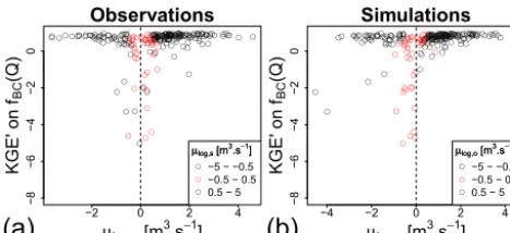
Figure 2. Values of KGE0 on log-transformed flows (a, b)
ver-sus the mean of the log-transformed observed and simulated flows compared. As a benchmark, the same plots are drawn with untrans-formed flows(c, d). Each dot represents the performance obtained in validation for one catchment after calibration with the KGE0on untransformed flows as an objective function. In plots(a)and(c), the axis values represent the observed log-transformed flow aver-ages and the color represents the simulated averaver-ages, while in plots
(b)and(d)it is the opposite.
by adding to flows a constant equal to 1/100 of the mean ob-served flows. The parameter of the Box–Cox transformation is fixed at the value of 0.25, as Vázquez et al. (2008) argue that it is an usual value in hydrological studies.
5 Results
5.1 Instability when the moments of log-transformed
flows become close to zero
Figure 2a and b analyse the stability of the KGE0 values with log-transformed flows obtained in the validation period. The KGE0 values were plotted against the mean of the log-transformed observed (a) and simulated (b) flows. When any of these means tends to be close to zero, the KGE0criterion exhibits unusually low values. This plot illustrates the prob-lem identified in Sect. 3.1. These very negative values may alter model evaluation. When working on a large set of catch-ments, they may also bias the calculation of the mean perfor-mance over the catchment set, by heavily weighting these outlier values. Figure 2c and d shows that the catchments with negative KGE0 values in Fig. 2a and b do not seem to exhibit any specific behaviour when evaluated with the KGE0 values on untransformed flows: the criterion values are not lower in these catchments than in other catchments.
Further-● ● ● ● ●●●● ●●●● ●●● ● ● ●● ●●● ●● ● ●●●●●● ●●●●●●●●●●●●●●● ●●●●● ● ●● ● ● ●●●● ●● ● ● ●● ●●● ● ● ● ● ● ● ●● ● ●●●● ●● ●● ●●●●●●●● ●●●●●●●●●● ● ●●● ● ● ● ● ●● ● ● ●●● ● ● ● ● ●●●●●● ●●● ● ● ●●●●●●● ●●●●●●●●●●●●●●●●●● ● ●●●●●●●●●●●●●●●● ● ● ●● ●●● ●●●● ● ●● ● ●●●● ● ● ● ● ● ● ● ● ● ●● ● ●●●●●●● ● ●● ● ● ●●● ●● ● ● ● ●● ●● ● ● ● ● ● ●● ● ●
−2 0 2 4
−8 −6 −4 −2 0
Observations
µlog,o [m3.s−1]
KGE' on Q
(a)
● ● ●µlog,s [m3.s−1] µlog,s [m3.s−1]
−5 − −0.5 −0.5 − 0.5 0.5 − 5
● ● ● ●●● ●●● ●●●● ●● ● ● ●●●● ●● ●● ● ●●● ●●●●● ●●●●●●●●●● ●●●●●●●●●● ● ● ●●●● ●● ● ● ● ●● ● ● ● ● ● ● ● ●●● ● ●●●●●● ●● ● ● ●●●●●●● ●● ●●●●●● ● ● ●●● ●● ●●●●●● ●● ●●● ● ● ●●●●●●●● ●●●●●●●●● ●●●●●●●●●● ●●●●●●●●●●●●●● ●●●●●●●●●●●● ● ● ● ●●●●●●●●● ●●●●●●●●● ● ●● ● ● ● ●● ● ● ●●●●●● ● ●●● ● ● ● ●● ● ● ● ● ●●● ●● ● ● ● ● ● ● ●● ●
−4 −2 0 2 4
−8 −6 −4 −2 0
Simulations
µlog,s [m3.s−1]
KGE' on Q
(b)
● ● ●µlog,o [m3.s−1] µlog,o [m3.s−1]
−5 − −0.5 −0.5 − 0.5 0.5 − 5
● ● ● ● ●● ● ● ● ● ● ● ● ● ● ● ●● ●●● ●● ● ●● ●●● ● ● ● ●●● ● ● ● ● ●● ●● ● ● ● ● ● ● ● ● ● ● ● ● ● ● ●● ● ●● ●●● ● ● ● ● ● ● ● ● ● ● ●● ● ●● ● ● ● ● ● ● ● ● ● ● ● ● ● ● ● ● ● ● ● ● ● ● ● ● ● ● ● ● ● ● ● ● ●●● ● ● ● ● ● ● ● ● ● ● ● ●● ● ●● ● ●● ● ● ● ● ● ●●● ● ●● ● ● ● ● ● ● ● ●● ● ● ● ●● ●● ● ● ●● ●●●● ● ● ● ● ● ● ● ● ●● ● ●● ● ● ● ● ● ●● ● ● ● ● ● ● ● ● ● ● ● ● ● ● ● ●●●● ● ●● ● ●● ● ● ●● ● ● ● ● ● ● ● ● ● ● ● ● ● ●●● ●
−2 0 2 4
−8
−6
−4
−2
0
µlog,o [m3.s−1]
KGE' on Q − 1
(c)
● ● ●µlog,s [m3.s−1] µlog,s [m3.s−1]
−5 − −0.5 −0.5 − 0.5 0.5 − 5
● ● ● ● ●● ● ● ● ● ● ● ● ● ● ● ●●●● ●● ●● ● ●●● ● ● ● ● ●●● ● ● ● ● ●● ●● ● ● ● ● ● ●●● ● ● ● ● ● ● ●● ● ●● ●●● ● ● ● ●● ● ● ● ● ● ●● ● ●● ● ● ● ● ● ● ● ● ● ● ● ● ●●● ● ● ● ● ● ● ● ● ● ● ● ● ● ● ● ● ●●●● ● ● ● ● ● ● ● ● ● ● ● ● ● ● ●● ● ●● ● ● ● ● ● ●●● ● ●● ● ● ● ● ● ● ● ●● ● ● ● ●● ●● ● ● ●● ●●●● ● ● ● ● ● ●●● ●● ● ●● ● ● ● ● ● ●● ● ● ● ●● ● ● ● ● ● ● ● ● ● ● ●●●● ● ●● ● ● ● ● ● ●● ● ● ● ● ● ● ● ● ● ● ● ● ● ●●● ●
−4 −2 0 2 4
−8
−6
−4
−2
0
µlog,s [m3.s−1]
KGE' on Q − 1
(d)
● ● ●µlog,o [m3.s−1] µlog,o [m3.s−1]
−5 − −0.5 −0.5 − 0.5 0.5 − 5
Figure 3.Values of KGE0on square-root(a, b)and inverse(c, d)
transformed flows versus the mean of the log-transformed observed and simulated flows. Each dot represents the performance obtained in validation for one catchment after calibration with the KGE0on untransformed flows as an objective function. In plots(a)and(c), the axis values represent the observed log-transformed flow aver-ages and the color represents the simulated averaver-ages, while in plots
(b)and(d)it is the opposite.
more, this result can be completed by making the same plot for other transformations, giving more weight to low flows. Figure 3 shows that square-root (Fig. 3a and b) and inverse (Fig. 3c and d) transformations do not encounter the same problems as with the logarithm for catchments that have an average log-transformed flow around zero.
The KGE0on log-transformed flows can also be compared to the NSE using the same transformation. Figure 4 shows that, when KGE0is significantly lower than NSE, the average of log-transformed flows (observed or simulated) is around zero (red dots in the figure). This tends to confirm that the strongly negative KGE0values stem more from a numerical issue than an actual problem in simulated values, because the NSE values in these catchments remain positive or around zero.
In this technical note, the impact of a near-zero standard deviation of log-transformed flows is not presented because it is rarer than near-zero mean values. The standard deviations of flows in the catchments studied are indeed all significantly higher than zero.
5.2 Dependence on the flow unit chosen
[image:4.612.313.546.67.283.2]● ● ● ● ● ● ●● ● ● ● ● ● ● ● ● ● ● ● ●● ● ● ● ● ● ● ●● ● ● ● ● ● ● ● ●● ● ● ● ● ●●● ● ● ● ● ● ● ● ● ● ●●●●● ● ● ● ●●●● ● ● ● ● ● ● ● ●● ● ● ● ● ● ●● ●●●● ● ● ● ● ● ● ● ● ●● ● ● ● ● ● ● ●● ● ● ● ● ● ● ● ● ● ● ● ● ●● ● ● ● ● ● ● ● ● ● ●●●●● ● ● ● ● ●●● ● ● ● ● ● ● ● ● ●● ●●●●● ● ● ●●● ●● ●●●●●● ●● ● ●● ● ● ● ● ● ● ●●●● ● ● ●●●● ●●●● ● ● ● ● ● ● ● ● ● ● ●● ● ●● ● ● ● ● ● ● ● ● ● ● ● ● ● ● ● ● ● ● ● ●●● ● ● ● ●
−6 −4 −2 0
−6 −4 −2 0 ● ● ● µlog,o [m3.s−1] µlog,o [m3.s−1] −5 − −0.5 −0.5 − 0.5 0.5 − 5
NSE on log(Q)
KGE' on log(Q)
(a)
● ● ● ● ● ● ●● ● ● ● ●● ● ● ● ● ● ● ●● ● ● ● ● ● ● ● ●● ● ● ● ● ● ● ● ●● ● ● ● ● ●●● ● ● ● ● ● ● ● ● ● ●●●●● ● ● ● ●●●● ● ● ● ● ● ● ● ●● ● ● ● ● ● ●● ●●●● ● ● ● ● ● ● ● ● ●● ● ● ● ● ● ● ● ● ● ● ● ● ● ● ● ● ● ● ● ● ● ●● ● ● ● ● ● ● ● ● ● ●●● ● ● ● ● ● ● ●●● ● ● ● ● ● ● ● ● ●● ●●●●● ● ● ●●● ●● ●●●●●● ●● ● ●● ● ● ● ● ●● ●●●● ● ● ●●●● ●●●● ● ● ● ● ● ●● ● ● ● ●● ● ● ● ● ● ● ● ● ● ● ● ● ● ● ● ● ● ● ● ● ● ● ●● ● ● ● ● ● ●−6 −4 −2 0
−6 −4 −2 0 ● ● ● µlog,s [m3.s−1] µlog,s [m3.s−1] −5 − −0.5 −0.5 − 0.5 0.5 − 5
NSE on log(Q)
KGE' on log(Q)
[image:5.612.50.283.67.173.2](b)
Figure 4.Comparison between KGE0and NSE values on the
valida-tion period using a calibravalida-tion with KGE0on untransformed flows as an objective function. The red dots represent the catchments where the average of log-transformed observed(a)or simulated(b)flows is around 0.
●●● ●● ●● ● ● ● ● ●●● ● ● ● ● ● ●●● ● ● ● ● ● ● ● ● ●●● ●● ●● ●● ●● ● ● ● ● ● ● ● ●●● ● ● ● ● ● ● ●● ●● ● ● ●●●● ● ●● ● ●● ● ● ●● ● ● ●●●●●●● ●●● ● ● ● ● ● ● ● ●● ● ● ● ● ●● ● ● ● ● ● ● ●●●●● ● ● ● ● ● ● ● ● ● ● ● ● ● ● ●●● ●●●●● ● ● ● ● ●●● ● ● ● ● ●● ●● ● ● ● ● ● ● ● ● ● ● ● ● ●● ● ●●●● ● ● ● ● ● ● ● ● ● ●●● ●● ● ● ● ● ● ● ● ● ●● ● ● ● ● ● ● ● ● ● ● ● ● ● ● ● ● ● ● ● ● ● ● ● ● ● ● ● ● ● ●● ● ●● ● ● ● ● ● ● ● ●●●●
−0.4 0.0 0.2 0.4 0.6 0.8 1.0
−0.4 0.0 0.2 0.4 0.6 0.8 1.0
KGE' on Q [m3.s−1]
KGE' on Q [l.
s − 1 ]
(a)
● ● ● ● ●● ● ● ● ● ● ● ● ● ● ● ● ● ● ● ● ● ● ● ● ● ● ● ● ● ● ● ● ● ●● ● ●● ● ● ● ● ● ● ● ● ● ● ● ● ● ● ● ● ● ● ● ● ● ● ●● ● ● ● ● ● ●● ● ● ● ● ● ● ● ● ● ● ● ● ● ● ● ● ● ● ● ● ● ● ● ● ● ● ● ● ● ● ● ● ● ●● ● ● ● ● ● ● ● ● ● ● ● ● ● ● ● ● ● ● ● ● ●● ●● ● ● ● ● ● ● ● ● ● ● ● ● ● ● ● ● ● ● ● ● ● ● ● ● ● ●● ● ● ● ● ● ● ● ● ● ● ● ● ● ● ● ● ● ● ● ● ● ● ● ● ● ● ● ● ● ● ●● ● ●● ● ● ● ● ● ● ● ● ● ●● ● ● ● ● ● ● ● ● ● ● ● ● ● ● ● ● ● ● ● ● ● ● ● ●−0.4 0.0 0.2 0.4 0.6 0.8 1.0
−0.4 0.0 0.2 0.4 0.6 0.8 1.0
KGE' on log(Q) [m3.s−1]
KGE' on log(Q) [l.
s
−
1 ]
[image:5.612.310.539.73.176.2](b)
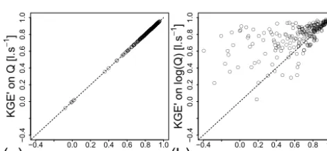
Figure 5. Dependence on flow units of the KGE0 using
untrans-formed flows (a)and log-transformed flows(b)in the 240 catch-ments. The parameters used for simulation evaluation were obtained by calibrating GR4J using KGE0on untransformed flows.
the KGE0on log-transformed flows in litres per second. Fig-ure 5b shows that, for the catchments tested, the values of KGE0 on log-transformed flows clearly depend on the flow unit used. A more optimistic evaluation of model perfor-mance will generally be obtained with the flows in litres per second. As a comparison, Fig. 5a shows that the KGE0with untransformed flows is not affected by the flow unit change. This dimension dependence makes the KGE0values based on log-transformed flows very difficult to interpret.
The higher model performance when using litres per sec-ond than when using square metres per secsec-ond can be ex-plained analytically. Considering Eq. (7), the formula of the bias ratio in litres per second regarding the averages in metres per second is as follows:
βlog[L s−1] =
log(1000)+µlog,s[m3s−1]
log(1000)+µlog,o[m3s−1]
. (8)
Because log(1000)is not negligible compared to the av-erages, adding this constant term would artificially improve
β and, by extension, the KGE0value. Theγ ratio is also af-fected and, due to the interactions between the standard devi-ation and the averages, modifies the KGE0value differently.
Qm/10 Qm/20 Qm/30 Qm/40 Qm/50 Qm/60 Qm/70 Qm/80 Qm/90 Qm/100
Mean NSE(log(Q)) Mean KGE'(log(Q))
−0.4
0.0
0.4
0.8
Fraction of mean flow (Qm) over the test period added
Efficiency v
[image:5.612.49.285.257.366.2]alue
Figure 6.Sensitivity of NSE and KGE0 to the fraction of average
flows that is added to flows to avoid zero flows in the logarithmic transformation for 240 catchments over the validation period. This graph is inspired by Fig. 9 in Pushpalatha et al. (2012).
5.3 Dependence on the value added to avoid the
zero-flow issue
Pushpalatha et al. (2012) showed that the sensitivity of the NSE criterion on log-transformed flows to the small added constant declines when this constant decreases (from 1/10 to 1/100 of the mean observed flow) and becomes limited for very small values (see Fig. 9 in Pushpalatha et al., 2012). We performed the same test with the KGE0criterion and we ob-tained a very different result (Fig. 6). The impact on perfor-mance is erratic for different values added to flows and does not show any trend. This may be due to the numerical issues shown in Sect. 5.1. For these reasons, the impact of added values can be major and may alter the model evaluation.
5.4 The case of the Box–Cox transformation
As presented in Sect. 3.3, instead of adding a small value to flows, a Box–Cox transformation can be applied to flows to mimic the logarithm transformation without the zero-flow problem. However, even though it removes the depen-dence of the KGE0 value to the value added to avoid zero flows, the other issues presented in the previous sections ex-ist as for the logarithm. For catchments in which the log-transformed flows’ average is close to zero, the Box–Cox transformed flows exhibit the same behaviour as with the logarithm (Fig. 7). This result is logical because the Box– Cox transformation of 1 is equal to 0, as for the logarithmic transformation.
The Box–Cox transformation is also dependent on the units (Fig. 8a). However, for this last issue, a slight modi-fication of the Box–Cox formula allows one to address this problem. The classical Box–Cox transformation can be writ-ten as follows:
fBC(Q)= Qλ−1
λ , (9)
● ●●●● ● ● ● ● ● ● ● ●● ● ● ● ●●● ●● ● ●●●●● ● ●● ●●●●● ● ● ● ● ● ● ● ● ● ● ● ● ● ● ● ● ● ● ● ●● ● ● ● ● ● ●● ● ● ● ● ● ● ● ● ● ● ● ●●●● ●● ● ● ● ● ● ●● ● ●● ● ● ● ● ● ● ● ● ● ● ● ● ● ● ● ● ● ● ● ● ● ● ● ● ● ● ● ● ● ● ● ● ● ●● ●● ● ● ● ● ●● ● ● ● ● ● ●●● ●● ●● ● ● ● ● ● ● ●● ● ● ● ●● ● ● ● ● ●● ●●●● ● ● ● ● ● ●● ● ● ● ●● ● ● ● ● ● ●● ●● ● ● ● ● ● ● ● ● ● ●● ●● ●● ● ● ● ● ● ● ●● ● ● ●● ● ● ● ● ● ● ●● ● ● ● ● ● ● ●● ● ●
−2 0 2 4
−8 −6 −4 −2 0 Observations
µlog,o [m3.s−1]
KGE' on f
B C (Q)
(a)
● ● ●µlog,s [m3.s−1]
µlog,s [m3.s−1]
−5 − −0.5 −0.5 − 0.5 0.5 − 5
● ●●●● ● ● ● ● ● ●● ●● ● ● ● ●● ●● ● ● ● ●● ● ● ●● ● ●●●● ● ● ● ● ● ● ● ● ● ● ● ●● ● ● ● ● ● ● ● ●● ● ● ● ● ● ●● ● ● ● ● ● ● ● ● ● ● ● ●●●● ●● ● ● ● ● ● ●● ● ●● ● ● ● ● ● ● ● ● ● ● ● ● ● ● ● ● ● ● ● ● ●● ● ● ● ● ● ● ● ● ● ● ● ●● ● ● ● ●● ● ●● ● ● ● ● ● ●● ● ●● ●● ● ● ● ● ● ● ●●● ● ● ●● ●● ● ● ●● ●● ● ● ● ● ● ● ●● ● ● ● ●●● ● ● ● ● ● ●● ●● ●● ● ● ● ● ● ● ●● ● ●●● ● ● ● ● ●● ● ● ● ● ● ●● ● ● ● ● ● ● ● ● ● ● ● ● ● ● ● ●● ●
−4 −2 0 2 4
−8 −6 −4 −2 0 Simulations
µlog,s [m3.s−1]
KGE' on f
B C (Q)
(b)
● ● ●µlog,o [m3.s−1]
µlog,o [m3.s−1]
−5 − −0.5 −0.5 − 0.5 0.5 − 5
Figure 7.Values of KGE0on Box–Cox transformed flows versus
the mean of the log-transformed observed (a)and simulated(b)
flows. Each dot represents the performance obtained in validation for one catchment after calibration with the KGE0on untransformed flows as an objective function. In plot(a), the axis values represent the observed log-transformed flow averages and the color represents the simulated averages, while in plot(b)it is the opposite.
● ● ● ● ● ● ● ● ● ● ● ● ●● ● ●●●● ● ● ● ● ● ● ● ● ● ● ● ● ● ● ●●● ● ● ● ● ● ● ●● ●●●● ● ● ● ● ● ● ● ● ● ●●● ● ● ● ● ● ●● ● ● ● ● ● ● ● ● ● ● ● ● ● ● ●● ● ●● ● ● ● ● ● ● ● ● ● ● ●● ● ● ● ● ● ● ● ● ● ● ● ● ● ●● ● ● ● ● ● ●● ●● ● ● ● ● ●● ● ● ● ● ● ● ● ● ● ●● ● ● ● ● ● ● ● ● ● ● ● ● ● ● ● ●● ● ● ● ● ● ● ● ● ● ● ● ● ● ● ● ● ● ● ● ● ● ● ●● ● ● ● ● ● ● ● ● ● ● ● ●● ● ● ● ● ● ● ● ● ● ● ● ● ● ● ● ● ● ● ● ● ● ● ●
−0.4 0.0 0.2 0.4 0.6 0.8 1.0
−0.4 0.0 0.2 0.4 0.6 0.8 1.0
KGE' on fBC(Q) [m3.s−1]
KGE' on f
B C (Q) [l. s − 1 ]
(a)
● ● ●●●● ● ● ● ● ● ● ● ● ●● ● ● ●● ● ● ● ● ● ● ● ● ● ● ● ● ● ● ● ● ●● ● ● ● ● ● ● ● ● ●●●● ●● ● ●● ● ● ● ● ● ●● ● ●● ● ● ● ● ● ● ● ●● ● ● ●●● ● ● ● ● ● ● ● ● ●● ●● ● ●●●● ● ● ● ● ● ● ● ●● ● ● ● ● ● ●● ● ● ● ● ● ● ●● ● ● ● ●● ● ● ●●● ● ● ●● ●● ● ● ●● ● ● ● ● ● ● ● ● ● ●● ●● ● ● ● ● ● ● ● ● ● ● ● ● ● ● ● ● ● ● ● ● ● ● ● ● ● ● ● ● ● ● ● ● ● ● ● ●● ● ●●● ● ●● ● ● ● ● ● ● ● ● ●●● ● ● ● ● ● ● ●● ● ● ● ● ● ● ● ● ● ●● ● ● ● ● ● ● ●−0.4 0.0 0.2 0.4 0.6 0.8 1.0
−0.4 0.0 0.2 0.4 0.6 0.8 1.0
KGE' on f'BC(Q) [m3.s−1]
KGE' on f'
[image:6.612.51.285.67.174.2]B C (Q) [l. s − 1 ]
(b)
Figure 8.Dependence on flow units of the KGE0using Box–Cox
transformed flows without adaptation (a, Eq. 9) and with adaptation (b, Eq. 10) in the 240 catchments. The parameters used for simula-tion evaluasimula-tion were obtained by calibrating GR4J using KGE0on untransformed flows.
Using this equation, the KGE0 on transformed flows will be unit-dependent because of the additive term 1 in the nu-merator. To avoid this, we can slightly modify the formula, by replacing the term 1 by a constant with a unit dependence (here we propose 1/100 of the mean flow) and by putting it to the powerλ:
fBC0 (Q)=Q
λ−(0.01µ
o)λ
λ . (10)
Using Eq. (10), the KGE0criterion remains dimensionless using the Box–Cox transformation (Fig. 8b).
Furthermore, because the zero of the modified Box–Cox function is not 1 any more, this transformation would reduce the issue of strongly negative values whenµlog,oorµlog,sare
around zero. However, there still is an issue if the average of simulated flows is around the zero of the modified Box–Cox function (i.e. ifµs=(0.01µo)λ, Fig. 9). This instability
oc-curs more rarely than for the logarithm transformation but can be more frequent if larger percentages of the average of observed flow or differentλvalue are used. Because this
in-● ● ● ●●● ● ● ●●●●●● ● ● ●●●● ●● ● ●● ●●● ● ●● ●●●● ● ● ● ●●●●● ● ● ● ●● ●● ● ● ● ●●●●● ●● ● ● ●● ●●● ● ● ● ●● ●● ● ● ●●●● ●● ● ● ● ●●● ●● ●● ● ●● ● ● ●● ● ● ● ● ●●● ● ● ● ● ● ●●●● ● ● ● ● ● ● ● ● ● ● ● ● ● ●● ● ● ●●●●●●● ●●●● ● ● ●● ● ● ●●● ●●●● ● ● ● ●●●●●●●●●●● ● ●● ● ●●●●●●●● ●● ● ● ● ● ● ● ● ●●● ● ● ● ● ●● ● ●●● ● ● ● ● ● ● ● ● ● ●● ● ● ● ●● ● ●
0 2 4 6 8
−8 −6 −4 −2 0 Observations
µf'BC,o [m
3.s−1]
KGE' on f'
B C (Q)
(a)
● ● ● µlog,s [m3.s−1] µlog,s [m3.s−1] −5 − −0.5 −0.5 − 0.5 0.5 − 5● ● ● ●●● ● ● ●● ●●●● ● ●● ●●● ●● ● ● ●●● ● ● ●●●● ●●●● ● ● ● ●●● ● ●● ● ●● ● ● ● ● ●●●●● ●● ● ● ● ●● ● ● ● ● ● ● ● ● ● ● ● ●●●● ●● ● ● ● ●● ●● ●●● ● ●●●●●● ● ● ● ●●● ● ● ● ● ● ●●●● ● ● ●● ● ● ● ● ● ● ● ● ● ● ● ● ● ●●●●●●● ●● ● ● ●●● ● ●● ●●● ●● ● ● ● ● ● ●● ●●●●●●●●● ● ● ● ●●●●●●●●●●● ● ● ●● ● ● ● ● ●● ● ●● ● ● ● ● ●●● ● ● ● ● ● ● ●● ●● ● ● ● ● ●● ●
0 2 4 6 8
−8 −6 −4 −2 0 Simulations
µf'BC,s [m
3.s−1]
KGE' on f'
B C (Q)
(b)
● ● ● µlog,o [m3.s−1] µlog,o [m3.s−1] −5 − −0.5 −0.5 − 0.5 0.5 − 5Figure 9.Values of KGE0on modified Box–Cox transformed flows
(Eq. 10) versus the mean of this transformed observed(a)and sim-ulated(b)flows. Each dot represents the performance obtained in validation for one catchment after calibration with the KGE0on un-transformed flows as an objective function. In plot(a), the axis val-ues represent the observed transformed flow averages and the color represents the simulated averages, while in plot(b)it is the oppo-site. ● ●●●●●● ● ● ● ● ● ●●●● ●●●●●●●●●● ● ●● ● ●● ●●● ● ● ● ●●● ●● ●●●●●●●●●●●●● ● ● ●●●●●●● ● ● ●● ● ● ●●●●● ●● ●●● ● ● ● ● ● ● ●● ● ● ● ● ● ●● ● ● ● ●●●● ●● ● ●●● ● ●●●●●●●● ● ● ● ●● ● ● ● ●●●●●●●●●●●●●●●●●● ●● ● ● ● ● ●●●● ● ●●●●● ● ●●●●● ● ●● ●● ● ●● ● ●●●●●● ● ● ● ● ● ● ●●●● ● ●● ● ● ● ● ● ● ●● ● ● ●● ●●● ●●● ●●● ● ● ● ● ● ● ● ● ●● ●● ● ● ●●●●
−6 −4 −2 0
−6 −4 −2 0 ● ● ● µlog,o [m3.s−1] µlog,o [m3.s−1] −5 − −0.5 −0.5 − 0.5 0.5 − 5
KGE' on fBC(Q)
KGE' on f'
B C (Q)
(a)
● ●●●●●● ● ● ● ● ● ●●● ●●●●●●●●●●● ● ●● ● ●● ●●● ● ●● ●●● ●● ●●●●●●●●●●●●● ● ● ● ●●●●● ● ● ● ● ●● ● ● ●●●●● ●●●●● ● ● ● ●● ● ●● ● ● ● ● ● ●● ● ● ● ●●●● ●● ● ●●● ● ●●●●●●●● ● ● ● ●● ● ● ● ●●●●●●●●●●●●●●●●●● ●● ● ●● ● ●●●● ● ●●●●● ● ●●● ●● ● ●● ●● ● ● ●● ● ●●●●●● ● ● ● ● ● ● ●●●● ● ●● ● ● ● ● ● ● ●● ● ● ●● ●●● ●●● ●●● ● ● ● ● ● ● ● ● ●● ●● ● ● ●●●●−6 −4 −2 0
−6 −4 −2 0 ● ● ● µlog,s [m3.s−1] µlog,s [m3.s−1] −5 − −0.5 −0.5 − 0.5 0.5 − 5
KGE' on fBC(Q)
KGE' on f'
B
C
(Q)
[image:6.612.312.546.68.175.2](b)
Figure 10. Comparison between KGE0 values on Box–Cox and
modified Box–Cox transformed flows on the validation period us-ing a calibration with KGE0on untransformed flows as an objective function. The red dots represent the catchments where the average of log-transformed observed(a)or simulated(b)flows is around 0.
stability is due toµs(which is only in the denominator of the γ ratio in Eq. 6), it will only affect the KGE0. The KGE is not affected because anαratio is used instead of theγ ratio (Eqs. 1 and 5).
The modified Box–Cox transformation (Eq. 10) allows unit dependence to be avoided and the instability issues due to the values of average flows to be reduced (especially when using the KGE). The behaviour of this modified transforma-tion also remains similar to the one of the initial Box–Cox transformation except whenµlog,oorµlog,s are around zero
(Fig. 10).
6 Summary
6.1 Log transformation should not be used in the KGE
or KGE0criterion
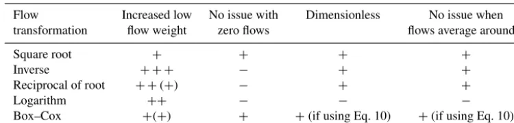
[image:6.612.312.545.288.397.2]Table 1.Pros (+) and cons (−) of different flow transformations to improve consideration of low flows in KGE0. In the second column, the number of+symbols represents the intensity of the low-flow weight increase. There are parentheses around the last+for inverted root and Box–Cox transformations because the low-flow weight depends on parameters.
Flow Increased low No issue with Dimensionless No issue when transformation flow weight zero flows flows average around 1
Square root + + + +
Inverse + + + − + +
Reciprocal of root + +(+) − + +
Logarithm ++ − − −
Box–Cox +(+) + +(if using Eq. 10) +(if using Eq. 10)
can lead to difficulties in the interpretation of criterion values. The criterion does not remain dimensionless like NSE with a prior logarithmic transformation. It also becomes overly sensitive when the log-transformed flows’ average becomes close to zero, yielding potentially very negative values, or when a small constant is added to flows prior to logarithmic transformation to cope with zero flows. Because of all these issues, logarithmic transformation should be avoided when using KGE0.
6.2 Alternatives
Instead of KGE0on log-transformed flows, several transfor-mations can be used to calculate KGE0. The pros and cons for several transformations are summarised in Table 1. The reciprocal of root (RoR) is an example of a transformation used in the literature that is not tested in the article but leads to an increase in the weight of low flows (Chapman, 1964; Ishihara and Takagi, 1965; Ding, 1966). As stated in Ding (2018b), it can be parametrized with the value of the power in the root (Q−N1). Depending on the value ofN, there will
be more or less weight on low flows (Ding, 2018a). The higher N is, the less the weight on low flows is. This N
value can also be determined with the recession curves of observed flows. Regarding this table, the modified Box–Cox transformation (Eq. 10) seems to be the best solution but it still faces instabilities for some flow average values (for the KGE0). Thus, there is no ideal solution to avoid all problems. Modellers have to make a choice depending on their specific applications. According to the intensity of low-flow weight increase that is needed, the choice of transformation has to be adapted. Garcia et al. (2016), for example, recommend av-eraging two KGE0criteria, computed on untransformed and inverted flows, into a composite criterion.
Note that many studies use NSE on log-transformed flows (see for example Lyon et al., 2017; Nguyen and Di-etrich, 2018). Fortunately, the mathematical formulation of NSE avoids all the problematic aspects identified for KGE with the logarithmic transformation. However, this may not be a sufficient argument to continue to use NSE given the is-sues presented by Gupta et al. (2009) and Schaefli and Gupta (2007):
– the underestimation of variability,
– the low weight of water balance errors for catchments with highly variable flows,
– the poor benchmark represented by the mean flows for catchments with highly variable flows.
6.3 Final remarks
Two additional remarks should be taken into account on this topic. First, as noted by Harald Kling in a personal commu-nication, 2018, prior transformations on flows in KGE (or in NSE) lead to a misinterpretation in the estimation of the water balance. The other components of the KGE also lose their initial physical meaning. KGE on transformed flows can give more information on low flows, but the physical inter-pretation of the criterion is not as simple as in the case of untransformed flows.
Secondly, even if it did not occur in our experiment, the issue described in this technical note may lead to problems during the calibration process. Indeed, it can create a strongly negative zone in the objective function hyperspace, which may negatively impact the performance of local calibration algorithms.
Data availability. The daily flow data can be downloaded from the Banque HYDRO website (http://www.hydro.eaufrance.fr/, last ac-cess 29 August 2018). The climatic data from the SAFRAN reanal-ysis used in this paper (daily precipitation and temperature) are not freely available. The data was provided to Irstea following a con-vention between the two institutes. However, the analyses can be reproduced using open data and would lead to similar conclusions.
Author contributions. LS made the technical development and the analysis. The paper was written by him, GT and CP.
Acknowledgements. The authors thank Météo France for providing the data used in this work. We also wish to thank Alban De Lavenne, Laure Lebecherel, Maria-Helena Ramos and Cedric Rebolho for the discussions on the different aspects of the issues using the logarith-mic transformation with KGE. We thank Andrea Ficchí for his work on the database and Linda Northrup for her correction of the English language of an earlier version of the paper. Finally, we extend our thanks to Harald Kling for discussions on this issue.
We thank the topical editor, Bettina Schaefli, for her careful reading of the paper, her suggestion on the modified Box–Cox transformation and the following discussions. We also thank the two reviewers, Lieke Melsen and Björn Guse, for taking the time to read our paper and for their remarks that helped us to make the paper and the figures more understandable. We thank Sivarajah Mylevaganam for the discussions that helped us to be more precise in the KGE and KGE0 description. Finally, we particularly want to thank John Ding for his suggestion to add the RoR transformation (that we did not know about before) to the article and for the fruitful discussions that followed.
Edited by: Bettina Schaefli
Reviewed by: Lieke Melsen and Björn Guse
References
Beck, H. E., van Dijk, A. I. J. M., de Roo, A., Mi-ralles, D. G., McVicar, T. R., Schellekens, J., and Brui-jnzeel, L. A.: Global-scale regionalization of hydrologic model parameters, Water Resour. Res., 52, 3599–3622, https://doi.org/10.1002/2015WR018247, 2016.
Box, G. E. P. and Cox, D. R.: An Analysis of Transformations, J. Roy. Stat. Soc. B, 26, 211–252, 1964.
Chapman, T. G.: Effects of groud-water storage and flow on the wa-ter balance, in: Proceedings of “Wawa-ter resources, use and man-agement”, 291–301, Australian Academy of Science, Melbourne Univ. Press, 1964.
Coron, L., Thirel, G., Delaigue, O., Perrin, C., and An-dréassian, V.: The suite of lumped GR hydrological mod-els in an R package, Environ. Model. Softw., 94, 166–177, https://doi.org/10.1016/j.envsoft.2017.05.002, 2017.
De Vos, N. J. and Rientjes, T. H. M.: Multi-objective perfor-mance comparison of an artificial neural network and a con-ceptual rainfall-runoff model, Hydrol. Sci. J., 52, 397–413, https://doi.org/10.1623/hysj.52.3.397, 2010.
Ding, J.: Interactive comment on “Technical note: Pitfalls in using log-transformed flows within the KGE criterion” by Léonard Santos et al., Hydrol. Earth Syst. Sci. Discuss., https://doi.org/10.5194/hess-2018-298-SC2, 2018a.
Ding, J.: Interactive comment on “Technical note: Pitfalls in using log-transformed flows within the KGE criterion” by Léonard Santos et al., Hydrol. Earth Syst. Sci. Discuss., https://doi.org/10.5194/hess-2018-298-SC5, 2018b.
Ding, J. Y.: Discussion of “Inflow hydrograph from large uncon-fined aquifers” by Ibrahim, H. A. and Brutsaert, W. J., J. Irrig. Drain. Am. Soc. Civ. Eng., 92, 104–107, 1966.
Ficchí, A., Perrin, C., and Andréassian, V.: Impact of temporal resolution of inputs on hydrological model performance: An
analysis based on 2400 flood events, J. Hydrol., 538, 454–470, https://doi.org/10.1016/j.jhydrol.2016.04.016, 2016.
Garcia, F., Folton, N., and Oudin, L.: Which objective function to calibrate rainfall–runoff models for low-flow index simulations?, Hydrol. Sci. J., 62, 1149–1166, https://doi.org/10.1080/02626667.2017.1308511, 2016. Gupta, H. V., Kling, H., Yilmaz, K. K., and Martinez, G. F.:
Decom-position of the mean squared error and NSE performance criteria: Implications for improving hydrological modelling, J. Hydrol., 377, 80–91, https://doi.org/10.1016/j.jhydrol.2009.08.003, 2009. Hogue, T. S., Sorooshian, S., Gupta, H., Holz, A., and Braatz, D.: A Multistep Automatic Calibration Scheme for River Forecasting Models, J. Hydrom-eteorol., 1, 524–542, https://doi.org/10.1175/1525-7541(2000)001<0524:AMACSF>2.0.CO;2, 2000.
Ishihara, T. and Takagi, F.: A study on the variation of low flow, Bulletin of the Disaster Prevention Research Institute, 15, 75–98, http://hdl.handle.net/2433/124698, 1965.
Klemeš, V.: Operational testing of hydrological simulation models, Hydrol. Sci. J., 31, 13–24, https://doi.org/10.1080/02626668609491024, 1986.
Kling, H., Fuchs, M., and Paulin, M.: Runoff conditions in the upper Danube basin under ensemble of cli-mate change scenarios, J. Hydrol., 424–425, 264–277, https://doi.org/10.1016/j.jhydrol.2012.01.011, 2012.
Krause, P., Boyle, D. P., and Bäse, F.: Comparison of different effi-ciency criteria for hydrological model assessment, Adv. Geosci., 5, 89–97, https://doi.org/10.5194/adgeo-5-89-2005, 2005. Leleu, I., Tonnelier, I., Puechberty, R., Gouin, P., Viquendi, I.,
Co-bos, L., Foray, A., Baillon, M., and Ndima, P.-O.: Re-founding the national information system designed to manage and give access to hydrometric data, La Houille Blanche, 1, 25–32, https://doi.org/10.1051/lhb/2014004, 2014 (in French).
Lyon, S. W., King, K., Polpanich, O., and Lacombe, G.: Assessing hydrologic changes across the Lower Mekong Basin, J. Hydrol.: Reg. Stud., 12, 303–314, https://doi.org/10.1016/j.ejrh.2017.06.007, 2017.
Nash, J. E. and Sutcliffe, J. V.: River flow forecasting through con-ceptual models. Part I – A discussion of principles, J. Hydrol., 10, 282–290, https://doi.org/10.1016/0022-1694(70)90255-6, 1970. Nguyen, V. T. and Dietrich, J.: Modification of the SWAT model to
simulate regional groundwater flow using a multicell aquifer, Hy-drol. Process., 32, 939–953, https://doi.org/10.1002/hyp.11466, 2018.
Oudin, L., Hervieu, F., Michel, C., Perrin, C., Andréassian, V., An-ctil, F., and Loumagne, C.: Which potential evapotranspiration input for a lumped rainfall–runoff model?, J. Hydrol., 303, 290– 306, https://doi.org/10.1016/j.jhydrol.2004.08.026, 2005. Oudin, L., Andréassian, V., Mathevet, T., Perrin, C., and Michel,
C.: Dynamic averaging of rainfall-runoff model simulations from complementary model parameterizations, Water Resour. Res., 42, W07410, https://doi.org/10.1029/2005wr004636, 2006. Pechlivanidis, I. G., Jackson, B., McMillan, H., and Gupta, H.: Use
of an entropy-based metric in multiobjective calibration to im-prove model performance, Water Resour. Res., 50, 8066–8083, https://doi.org/10.1002/2013WR014537, 2014.
Pushpalatha, R., Perrin, C., Moine, N. L., and Andréassian, V.: A review of efficiency criteria suitable for evaluat-ing low-flow simulations, J. Hydrol., 420–421, 171–182, https://doi.org/10.1016/j.jhydrol.2011.11.055, 2012.
Quesada-Montano, B., Westerberg, I. K., Fuentes-Andino, D., Hidalgo, H. G., and Halldin, S.: Can climate variability in-formation constrain a hydrological model for an ungauged Costa Rican catchment?, Hydrol. Process., 32, 830–846, https://doi.org/10.1002/hyp.11460, 2018.
Schaefli, B. and Gupta, H. V.: Do Nash values have value?, Hy-drol. Process., 21, 2075–2080, https://doi.org/10.1002/hyp.6825, 2007.
Seeger, S. and Weiler, M.: Reevaluation of transit time dis-tributions, mean transit times and their relation to catch-ment topography, Hydrol. Earth Syst. Sci., 18, 4751–4771, https://doi.org/10.5194/hess-18-4751-2014, 2014.
Vázquez, R. F., Willems, P., and Feyen, J.: Improving the pre-dictions of a MIKE SHE catchment-scale application by us-ing a multi-criteria approach, Hydrol. Process., 22, 2159–2179, https://doi.org/10.1002/hyp.6815, 2008.