Measurement Error for Age of Onset in Prevalent Cohort Studies

http://dx.doi.org/10.4236/am.2014.511160

Measurement Error for Age of Onset in

Prevalent Cohort Studies

Yujie Zhong, Richard J. Cook

Department of Statistics and Actuarial Science, University of Waterloo, Waterloo, Canada Email: zyujie@uwaterloo.ca, rjcook@uwaterloo.ca

Received 11 March 2014; revised 20 April 2014; accepted 27 April 2014 Copyright © 2014 by authors and Scientific Research Publishing Inc.

This work is licensed under the Creative Commons Attribution International License (CC BY).

http://creativecommons.org/licenses/by/4.0/

Abstract

Prevalent cohort studies involve screening a sample of individuals from a population for disease, recruiting affected individuals, and prospectively following the cohort of individuals to record the occurrence of disease-related complications or death. This design features a response-biased sampling scheme since individuals living a long time with the disease are preferentially sampled, so naive analysis of the time from disease onset to death will over-estimate survival probabilities. Unconditional and conditional analyses of the resulting data can yield consistent estimates of the survival distribution subject to the validity of their respective model assumptions. The time of disease onset is retrospectively reported by sampled individuals, however, this is often associated with measurement error. In this article we present a framework for studying the effect of mea-surement error in disease onset times in prevalent cohort studies, report on empirical studies of the effect in each framework of analysis, and describe likelihood-based methods to address such a measurement error.

Keywords

Disease Onset Time, Left Truncation, Measurement Error, Model Misspecification, Prevalent Cohort

1. Introduction

disease onset to death. The prevalent cohort design features a form of response-dependent sampling, however, in the sense that diseased individuals with long survival times are preferentially selected for inclusion into the co-hort [1] [2] [7]; some authors refer to the resulting data as “length-biased”. Valid statistical inference depends critically on adequately addressing the sampling scheme in the likelihood construction, and there are two broad frameworks for analysis, both of which make use of the retrospectively reported time of disease onset recorded at the time of sampling.

Analysis in the conditional framework is based on the fact that individuals who died before the time of screening cannot be sampled, and so the survival times among sampled individuals are left-truncated by the time from disease onset to enrollment. The unconditional framework is based on the density of the survival times de-rived under the prevalent cohort sampling scheme. That is, if the disease incidence is stationary, the onset times follow a time homogeneous Poisson process, and the resulting left truncation times have a constant density. If the probability that an individual is sampled is proportional to their survival time, the density of times subject to this sampling scheme can be derived and used for likelihood construction.

For the conditional approach, parametric, nonparametric and semiparametric methods are relatively straight- forward and have seen considerable application [3] [8] [11]. Wang [10] proposed a product-limit estimator for left-truncated survival times which maximizes the conditional likelihood and loses no information when the dis-tribution of the truncation time variable is unspecified. For semiparametric Cox models, the partial likelihood approach can be adopted for left-truncated data but with an adjusted risk set [8] [11] [12]. Wang et al.[12] ar-gued that the nonparametric and semiparametric estimators are efficient when the distribution of the truncation time is unspecified but can be inefficient when the distribution of truncation time is parameterized.

Unconditional analyses [5] [13]-[16] are based on the joint distribution of the backward recurrence time (time from disease onset to sampling) and the forward recurrence time (time from sampling to death). Vardi [13] [14] and Asghrian et al. [5] developed the nonparametric maximum likelihood estimator (NPMLE) for right-cen- sored length-biased survival times, but this NPMLE does not have closed form and its limiting distribution is in-tractable [15] [16]. Huang and Qin [17] derived a new closed-form nonparametric estimator that incorporates the information about the length-biased sampling. Wang [18] proposed pseudo-likelihood for length-biased failure times under the Cox proportional hazards model, but this method cannot be applied to right-censored failure times. Luo and Tsai [19] and Tsai [20] derived pseudo-partial-likelihood estimators for right-censored length- biased data which have closed-form and retain high efficiency. Shen et al. [21] considered modeling covariate effects for length-biased data under time transform and accelerated failure time models. Qin and Shen [22] re-cently proposed two estimating equations for fitting the Cox proportional hazards model that are formulated based on different weighted risk sets.

Both conditional and unconditional analyses make use of the retrospectively reported times of disease onset, with the latter further based on the assumption of a stationary (Poisson) incidence process. However, there is of-ten considerable error and uncertainty in the retrospectively reported onset times. This is particularly true for onset times related to disease featuring cognitive impairment or mental health disorders. In some settings the reported times may better represent times of symptom onset, rather than the actual start of the disease process which may lead to underestimation of disease duration. In other settings the errors may lead to earlier or later reported onset times.

The purpose of this article is to examine the impact of measurement error in the retrospectively reported onset time for both the conditional and unconditional frameworks. The remainder of the paper is organized as follows. In Section 2, we introduce notation and likelihood construction for prevalent cohort data. The impact of misspe-cification of the disease onset time is explored in Section 3 by simulation for the unconditional and conditional approaches, and methods for correcting for this measurement error are described in Section 4. General remarks and topics for further research are given in Section 5.

2. Approaches to Statistical Analysis

2.1. Notation and Likelihood Construction

time of disease onset and Vi1 be the calendar time of death (time of entry to state D2); then Ti=Vi1−Vi0 de-notes the time of interest.

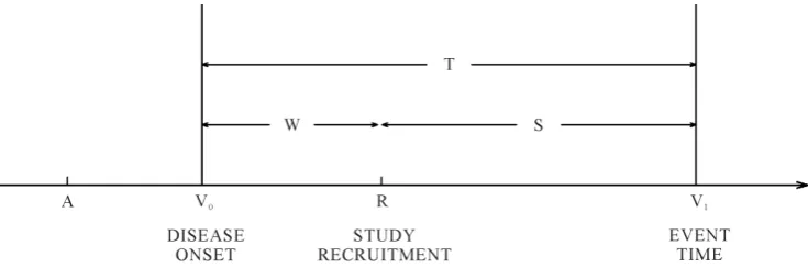
Consider a study starting at calendar time R (recruitment time), when individuals in the population are screened for the disease of interest and those who are diseased are to be recruited into the study.Figure 1 shows a hypothetical situation in the prevalent cohort study, where calendar time is represented on the horizontal axis. Individuals who are sampled must have developed the disease of interest at some point over the calendar time interval

[

A R,

]

, and be still alive at the recruitment time R. Those who develop the disease over

[

A R,

]

but die before the recruitment time cannot, of course, be selected for inclusion in the sample. Those who develop the disease after the recruitment time are also not eligible for recruitment. The times Wi = −R Vi0 and S=Vi1−R are called the backward and forward recurrence times for individual i respectively, and Ti=Wi+Si is the sur-vival time of interest. To accommodate incomplete follow-up, let Ci denote the right censoring time for indi-vidual i from disease onset, and Xi=min

(

T Ci, i

)

denote the survival time from disease onset; δi=I

(

Ti1<Ci

)

is a indicator of whether death is observed.

Let fT

( )

t;θ and T

( )

t;θ be the so-called unbiased probability density and survivor functions for Ti, which characterize the distribution in the target population, where a p×1 parameter vector θ indexes the distribution. The relevant density function for the observed left-truncated survival data for individual i is

(

0 0

)

₍

( )

₎

0 ;

, ; .

; T i

i i i i

T i

f t f t v T R v

R v

θ θ

θ

> − =

−

 (1)

The conditional likelihood for right-censored left-truncated survival data is

( )

(

0 0

)

(

₍

)

1

(

₎

)

1 0

; ;

, ; ,

;

i i

n

T i T i

C i i i i

i T i

f x x

L f x v T R v

R v

δ _θ δ _θ

θ θ

θ

−

=

∝ > − =

−

∏

_  (2)

assuming vi0 is recorded correctly. By conditioning on the observed truncation time, it is not necessary to model the distribution of the onset times.

If the disease onset process is a stationary Poisson process, f0

( )

v0 =1

(

R−A

)

and the resulting sample is right-censored length-biased sample. If the distribution of the onset time is known and can be parameterized, the conditional approach may be inefficient and it is natural to want to make use of the information contained in the onset process.

We now consider the distribution of the onset times over the interval

[

A R,

]

in the target population. Let

( )

(

)

0 0 d 0 0 0 0 d 0 0

f v v =P v ≤V ≤ +v v A V≤ ≤R be the probability an onset time occurs in an interval

[

v v0, 0+dv0

]

given it happens over

[

A R,

]

. We assume T⊥V0, so that the distribution of the survival time since disease on-set does not depend on onon-set time. We also define the sample onon-set time density for individuals who satisfy the inclusion criterion,

(

)

(

)

( ) (

)

( ) (

)

0 0 0

*

0 0 0 0 1

0

;

; , .

; d T

R

T A

f v R v

f v f v A V R V R

f u R u u

θ θ

θ −

= ≤ ≤ > =

−

∫



 (3)

[image:3.595.129.497.582.704.2]

When the onset process is stationary, as A→ −∞, the sample density function for the onset time (3) can be simplified to be

(

)

(

0

)

*

0 0

;

; T R v

f v θ θ

µ −

= (4)

where

[ ]

( )

0 ; d

E T tf t t

µ= =

_∫

∞ θ is the population mean survival time with disease.

From (3) and (4), one can see that the onset time among sampled individuals contains information regarding the survival distribution. The unconditional likelihood utilizing this information is based on the joint distribution of

(

V X0,

)

, which can be written as

( )

(

)

(

)

(

₍

) (

₎

)

( )

( )

0 0 1

1 1 * 0 0 1 0 , , ; ; ; ; ; i i n

F i i

i n

T i T i

i

i T i

M C

L f v x A V R V R

f x x

f v R v L L δ δ θ θ θ θ θ θ θ θ = − = ∝ ≤ ≤ ≥ = − = ×

∏

∏

_  (5)

where

( )

*

(

)

0 0

1 ;

n

M i i

L θ =

∏

₌ f v θ . Thus the full likelihood is the product of the conditional likelihood and the marginal likelihood of sample onset times, LM

( )

θ indexed by θ.

Under the assumption of a stationary disease process and based on (4), the unconditional likelihood for right- censored length-biased sample can be written as

( )

(

)

(

)

1 1 ; ; . i i n

T i T i

F i

f x x

L δ δ θ θ θ µ µ − =     = _  _{ } _    

∏

 (6)

Thus the unconditional approach exploits information in the disease onset times to improve efficiency over the conditional approach, but it does so by making stationary assumption for the disease onset process, which makes it less robust.

The estimators ˆθC and ˆθF can be found by maximizing the conditional (2) or unconditional (5) likelihoods respectively when parametric models are applied. Further, the resulting estimators have an asymptotic normal distribution, so

(

_ˆ

)

(

1

)

(

_ˆ

)

(

1

)

0, , 0, ,

D D

C C F F

n θ −θ →N − n θ −θ →N −

where C and F are the Fisher information matrices for conditional and unconditional likelihoods.

2.2. Nonparametric Estimation of the Survival Function Estimation

Nonparametric methods are often more appealing than parametric methods when there is limited knowledge re-garding the distribution of survival times. Wang et al. [23] and Wang [10] derived the product-limit estimator for left-truncated survival data. Let Y ui

( )

=I

(

Li< <u Ci

)

indicate whether individual i has been recruited into the study and under observation at time u, where Li= −R vi0 is the left-truncation time, and let

( ) (

)

† I

i i

Y u = u≤T be an indicator they are at risk of an event. Let dN ui

( )

=I

(

Ti=u

)

be the event indicator,

and

( )

( )

0d

u

i i

N u =

∫

N s . Then the logarithm of the likelihood for left-truncated data (2), can be rewritten as

( )

( )

( )

( ) ( )

{

0 0

}

1

d log d d

n

C i i i

i

l ∞Y u N u u ∞Y u u

=

=

∑ ∫

Λ −

_∫

Λ

where Y ui

( )

=Y u Yi

( ) ( )

i† u and Λ

( )

u is the cumulative hazard function. The nonparametric maximum like-lihood estimator (NPMLE) of the survivor function for right-censored left-truncated data is

( )

{

( )

}

ˆ _{1 d}ˆ _,

u t

t u

≤

=

∏

− Λ

 (7)

where dΛˆ

( )

u =dN u Y u⋅

( ) ( )

⋅ ,

( )

1

( )

n i i

Y u_⋅ =

∑

₌Y u , and dN u_⋅

( )

=

∑

n_i=1Y u_i

( )

dN u_i

( )

.

( )

( )

1 1

1

d d .

i i

i

n

i _{x x}

i

G x x G x

δ

δ ₋ −

≥ =

 

 

  _ _

∏

∫

(8)

Vardi [14] also argued that, based on the renewal theory, the joint distribution of

(

T V, 0

)

under length-biased sampling is f t

( )

µ. Hence the density function for the observed length-biased event time is

( )

( )

dG t =t F td µ, and then the survivor function for event time in the population is

( )

1

( )

d

t

t =

∫

∞ −u µ G u

 .

The full likelihood (6) under length-biased sampling can be rewritten as

( )

( )

( )

(

)

(

( )

)

( )

(

( )

)

1 1 1 1 1 1 1 1 1 d d d

d d ,

i i i i i i i i n i i F i

n i i _x

i n

i _x

i

F x x

L

x G x u G u

G x u G u

δ δ δ δ δ δ µ µ µ µ − = − ∞ − − = − ∞ − = = =   ∝ _{ }

∏

∫

∏

∏

∫



which is exactly the same as Vardi (8). The Vardi [14] algorithm can therefore be used to obtain the NPMLE of

( )

dG t , and by using the relationship between dF t

( )

and dG t

( )

, the NPMLE of dF t

( )

can be easily ob- tained by _ˆ

( )

1 _ˆ

( )

1 _ˆ

( )

dF t =t−dG t

∫

t−dG t .

Qin et al. [24] developed an expectation-maximization algorithm for the analysis of length-based data by con-structing a complete data likelihood using the Turnbull [9] approach and considering contributions from “ghosts”; these are individuals not sampled into the cohort because they died before the screening assessment. Unlike Vardi [14] method, their likelihood function is derived from the unbiased distribution of event time and EM algorithm directly estimates dF t

( )

, which allows one to impose any model and parameter constraints for this distribution function.

3. Error in the Reported Onset Time

3.1. Introduction

Both the conditional and unconditional analyses make use of the reported onset time, and the latter requires the additional assumption of a stationary disease incidence process. For individuals determined to have the disease at the time of assessment, the disease may have begun several years earlier, making accurate recall of the onset time difficult. There may therefore be considerable uncertainty about the reported onset time and the difference between the true onset time and the reported onset time represents recall, reporting, or measurement error; we will henceforth use the term measurement error.

Both the conditional and unconditional approaches to the analysis of prevalent cohort data will in general lead to biased estimators in the presence of measurement error. We therefore investigate the impact of this measure-ment error in both the conditional and unconditional frameworks for parametric and nonparametric settings.

3.2. The Classical Measurement Error Model

In retrospective studies, selected patients need to recall their disease onset times. In this case, the recall times are very likely different from the exact disease onset times, even though perhaps they are quite close. Consider dis-ease incidence over

[

A R,

]

, and a sample of the prevalent cohort is selected at recruitment time R. Let V0 be the exact disease onset time which is not observed and U0 be the retrospectively reported disease onset time. A classical error model Carroll et al. [25] leads to

0 0

U =V + (9) where N

(

0,σ2

)

is random measurement error, and A≤V0≤R.

trun-cated normal distribution, with density function written as g u v

(

0 0;φ

)

, suppressing the condition A U≤ 0≤R,

(

)

₍

(

₎

0 0

₍

)

₎

0 0

0 0

; ;

; ;

f u v g u v

F R v F A v

φ φ

φ φ

− =

− − −



 

(10)

where f_

( )

⋅;φ and F_

( )

⋅;φ are the density and cumulative distribution functions of  with parameter log

φ= σ, where σ is the standard deviation; we let ψ =

(

θ φ ′′ ′,

)

denote the vector of all parameters.

3.3. Empirical Study of Measurement Error

If we ignore the measurement error and treat U0 as the true onset time, both the left-truncation time and sur-vival time will be in error. Conditional and unconditional parametric analyses will lead to biased estimators for parameters of interest. To examine this impact, we conduct the following simulation study which follows the same strategy of Huang and Qin (2011) to generate length-biased data. We let the true disease onset time V0 be uniformly distributed over

[

A R,

] [

= 0,100

]

, and the underlying survival time T be independently generated from a Weibull distribution with survival function T

( )

t; exp

(

( )

t

)

κ

θ = − λ

 ; θ=

(

log , logλ κ ′

)

, and consider 0.5

λ= and κ =2. Hence the event happens at V1=V0+T at the calender time scale which can be recorded. Suppose the censoring time, measured from the time of recruitment, is independently and uniformly distributed over

[ ]

1, 2 , which leads to a 30% true censoring rate. To incorporate the measurement error in the onset time, we adapt the classical measurement error model (9) and assume that N

(

0,σ2

)

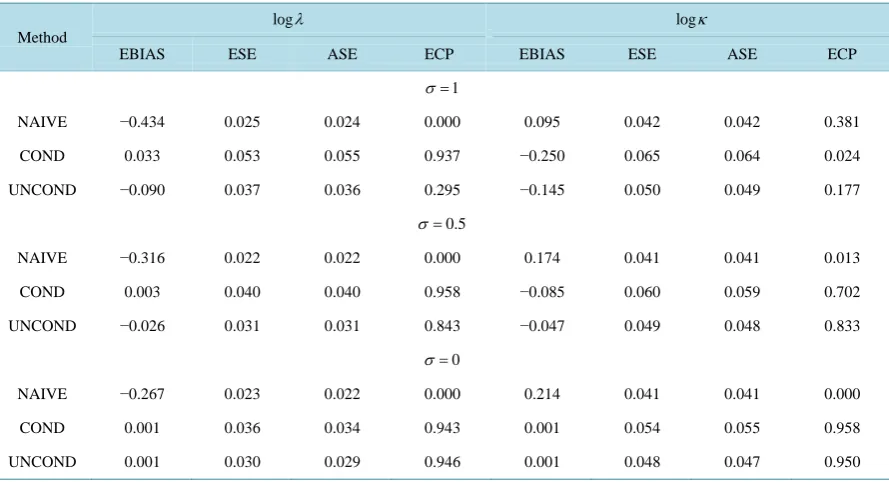
with σ =0.5 or 1.0 to re-flect mild and strong measurement error, respectively. In presence of measurement error, although the ascer-tainment criteria is still V1>R to form a prevalent cohort sample, both the left truncation time and survival time are affected by the random error and are recorded as R U− 0 and V1−U0, respectively. We set the sample size as n = 500 and simulation nsim = 1000 data sets. To examine the impact of measurement error in disease onset time, naive, conditional and unconditional parametric and nonparametric approaches are applied to the re-sulting data, all of which involved treating U0 as the “true” onset time.Table 1 summarizes the average bias (EBIAS), empirical standard error (ESE), average model-based standard error (ASE), and empirical 95% cov-erage probability of estimators based on naive (NAIVE), conditional (COND) and unconditional (UNCOND) likelihoods.

[image:6.595.92.537.481.722.2]

FromTable 1, we see that all three likelihood methods lead to biased estimators, since they all ignore the measurement error in the disease onset time. Although the ESE and ASE agree with each other, the empirical

Table 1. Empirical properties of estimators in presence of measurement error in disease onset time using Naive likelihood (NAIVE), Conditional likelihood (COND) and Unconditional likelihood (UNCOND); n = 500, nsim = 1000.

Method

logλ logκ

EBIAS ESE ASE ECP EBIAS ESE ASE ECP

1

σ =

NAIVE −0.434 0.025 0.024 0.000 0.095 0.042 0.042 0.381

COND 0.033 0.053 0.055 0.937 −0.250 0.065 0.064 0.024

UNCOND −0.090 0.037 0.036 0.295 −0.145 0.050 0.049 0.177

0.5

σ =

NAIVE −0.316 0.022 0.022 0.000 0.174 0.041 0.041 0.013

COND 0.003 0.040 0.040 0.958 −0.085 0.060 0.059 0.702

UNCOND −0.026 0.031 0.031 0.843 −0.047 0.049 0.048 0.833

0

σ =

NAIVE −0.267 0.023 0.022 0.000 0.214 0.041 0.041 0.000

COND 0.001 0.036 0.034 0.943 0.001 0.054 0.055 0.958

[image:7.595.92.537.372.721.2]

coverage probability is far away from the nominal value. Further, when the variance of the measurement error becomes smaller, the biases of estimators reduce a lot and the empirical coverage probabilities become better. This makes sense because the smaller the variance of measurement error, the closer of reported onset time to the true onset time, which reduces the impact of using the reported onset time.

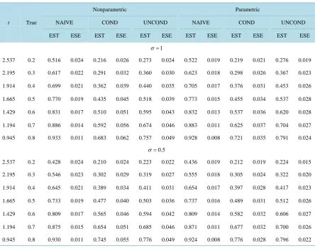
Table 2andTable 3 summarize the nonparametric estimates of the survivor functions and percentiles based on naive, conditional and unconditional approaches, along with the estimates based on parametric models for comparison. Similar conclusions can be drawn about the effect of measurement error in disease onset time for nonparametric analyses. One thing needs to mention is that even when the variance of measurement error be-comes smaller, the biases are still quite large for the naive approach, under parametric and nonparametric ana-lyses. This is because the naive approach treats the recruited sample as a representative sample of the population and does not correct for the selection bias for left-truncated or length-biased data.

To clearly understand the importance of correcting for measurement error in disease onset time for prevalent cohort samples, we plot the true survivor function versus estimated survivor functions based on the naive, condi-tional and uncondicondi-tional likelihoods without correcting for measurement error, both parametric and nonparame-tric models are considered.Figure 2 shows that ignoring the measurement error in onset time, both conditional and unconditional likelihoods lead to biased estimate of survivor function.

4. The Corrected Likelihood

4.1. Corrected Parametric Conditional Likelihood

A “correct” likelihood approach can be used to account for the measurement error in the onset time and will

Table 2. Empirical properties of nonparametric and parametric survivor estimators at certain time points based on naive (NAIVE), conditional (COND) and unconditional (UNCOND) likelihoods; n = 500, nsim = 1000.

t True

Nonparametric Parametric

NAIVE COND UNCOND NAIVE COND UNCOND

EST ESE EST ESE EST ESE EST ESE EST ESE EST ESE

1

σ =

2.537 0.2 0.516 0.024 0.216 0.026 0.273 0.024 0.522 0.019 0.219 0.021 0.276 0.019

2.195 0.3 0.617 0.022 0.291 0.032 0.360 0.030 0.623 0.018 0.298 0.026 0.367 0.023

1.914 0.4 0.699 0.021 0.362 0.039 0.440 0.035 0.705 0.017 0.376 0.031 0.453 0.026

1.665 0.5 0.770 0.019 0.435 0.045 0.518 0.039 0.773 0.015 0.455 0.034 0.537 0.028

1.429 0.6 0.831 0.017 0.510 0.051 0.595 0.043 0.832 0.013 0.537 0.036 0.620 0.028

1.194 0.7 0.886 0.014 0.592 0.056 0.674 0.046 0.883 0.011 0.625 0.037 0.704 0.027

0.945 0.8 0.933 0.011 0.683 0.062 0.757 0.049 0.928 0.008 0.721 0.035 0.791 0.024

0.5

σ =

2.537 0.2 0.428 0.024 0.210 0.024 0.223 0.022 0.436 0.019 0.212 0.019 0.224 0.015

2.195 0.3 0.546 0.023 0.302 0.029 0.319 0.027 0.555 0.018 0.305 0.024 0.322 0.020

1.914 0.4 0.645 0.021 0.389 0.034 0.411 0.031 0.654 0.017 0.397 0.028 0.417 0.023

1.665 0.5 0.733 0.019 0.477 0.040 0.503 0.036 0.737 0.016 0.489 0.031 0.512 0.026

1.429 0.6 0.809 0.017 0.565 0.046 0.594 0.042 0.809 0.014 0.582 0.032 0.606 0.027

1.194 0.7 0.875 0.015 0.654 0.051 0.685 0.046 0.871 0.011 0.677 0.032 0.700 0.026

[image:8.595.91.540.110.683.2]

Table 3. Empirical properties of nonparametric and parametric percentile estimators based on naive (NAIVE), conditional (COND) and unconditional (UNCOND) likelihoods; n = 500, nsim = 1000.

q

t True

Nonparametric Parametric

NAIVE COND UNCOND NAIVE COND UNCOND

EST ESE EST ESE EST ESE EST ESE EST ESE EST ESE

1

σ =

0.05

t 0.453 0.823 0.068 0.175 0.143 0.240 0.154 0.800 0.048 0.291 0.049 0.395 0.046

0.10

t 0.649 1.118 0.064 0.317 0.174 0.433 0.173 1.110 0.054 0.460 0.064 0.598 0.058

0.25

t 1.073 1.732 0.069 0.735 0.195 0.948 0.158 1.752 0.058 0.873 0.086 1.067 0.073

0.50

t 1.665 2.590 0.084 1.445 0.167 1.710 0.133 2.613 0.066 1.532 0.101 1.772 0.081

0.75

t 2.355 3.581 0.117 2.360 0.141 2.632 0.126 3.582 0.093 2.390 0.103 2.646 0.079

0.90

t 3.035 4.519 0.182 3.296 0.140 3.538 0.120 4.513 0.136 3.311 0.112 3.548 0.082

0.95

t 3.462 5.056 0.247 3.877 0.156 4.087 0.132 5.087 0.169 3.921 0.132 4.132 0.094

0.5

σ =

0.05

t 0.453 0.824 0.064 0.248 0.157 0.303 0.159 0.788 0.043 0.398 0.051 0.434 0.044

0.10

t 0.649 1.086 0.057 0.433 0.183 0.518 0.162 1.066 0.046 0.588 0.062 0.632 0.053

0.25

t 1.073 1.609 0.056 0.914 0.162 1.006 0.130 1.625 0.049 1.014 0.075 1.069 0.063

0.50

t 1.665 2.321 0.066 1.591 0.136 1.664 0.125 2.352 0.053 1.635 0.080 1.695 0.066

0.75

t 2.355 3.139 0.093 2.370 0.113 2.424 0.116 3.148 0.071 2.385 0.079 2.437 0.062

0.90

t 3.035 3.921 0.146 3.117 0.117 3.158 0.137 3.898 0.103 3.144 0.087 3.180 0.064

0.95

t 3.462 4.371 0.202 3.582 0.137 3.615 0.137 4.355 0.127 3.630 0.103 3.651 0.074

(a) (b)

yield unbiased estimators of the parameters of interest if the component model assumptions are correctly speci-fied. Such a likelihood should be based on the reported onset time and the (possibly censored) survival time, which will require explicit modeling of the measurement error process. Let h v u

(

1 0

)

be the density function of the calendar time of death given the reported onset time, i.e.

(

)

(

)

(

)

(

)

( )

(

)

(

)

( )

1 0 1 0 0 0 1

1 0 0 0 0 0 0

0 0 0 0 0 0

; , , , ;

; ; d

; ; d

R T A R T A

h v u P v u A U V R V R

f v v g u v f v v

R v g u v f v v

ψ ψ θ φ θ φ = ≤ ≤ ≥ − = −

∫

∫

 (11)

The “correct” conditional likelihood for right-censored left-truncated data

{

ui0, , ;xi δi i=1,,n

}

is of the form

( )

(

)

(

)

( )

(

)

( )

(

)

( )

(

)

(

)

( )

0 0 0 0 0 0

*

1

0 0 0 0 0 0

1

0 0 0 0 0 0

0 0 0 0 0 0

; ; d

( ; ) ; d

( ; ) ; d

; ; d

i

i

R n

T i i i i i i

A

C R

i

T i i i i i

A R

T i i i i i i

A R

T i i i i i

A

f x v g u v f v v L

R v g u v f v v

x v g u v f v v

R v g u v f v v

δ δ θ φ ψ θ φ θ φ θ φ = −  ₋    = _{ } −      ₋     ×_{ }  −    _

∫

∏

∫

∫

∫

   (12)

Similarly, the joint density of the observed onset time and calendar time of death is

(

)

(

)

(

₍

)

(

₎

)

(

)

(

)

( )

(

) ( )

(

)

0 0 1 1 0

1 0 1 0 0 0 0 1

0 0 1

0 0 0 0 0 0

1 0

0 0 0 0

, , ;

, ; , , , , ;

, ,

; ; d

; . ; d R T A R T A

P u A V R V R h v u h v u P v u u A U V R V R

P A U R A V R V R R v g u v f v v

h v u R v f v v

ψ ψ θ φ ψ θ ≤ ≤ ≥ = ≤ ≤ ≥ = ≤ ≤ ≤ ≤ ≥ − = −

∫

∫

  (13)

where the last equality is derived by (10).

The “correct” unconditional likelihood can then be constructed as follows,

( )

( )

( )

* * *

,

F M C

L ψ =L ψ ×L ψ 14) where

( )

(

)

(

)

( )

(

) ( )

0 0 0 0 0 0

*

1

0 0 0 0

; ; d

.

; d

R n

T i i i i i

A

M R

i

T i i i

A

R v g u v f v v

L

R v f v v

θ φ ψ θ =  ₋    =_{ } −  

∫

∏

∫



 (15)

Since L*M might contain the information about parameters we are interested in, the “correct” unconditional likelihood might be more efficient than the “correct” conditional likelihood. Further, when the underlying onset time is a stationary process, then we can let f0

( ) (

v0 R A

)

1

−

= − and let A→ −∞ to obtain both “correct” like-lihoods for length-biased data.

The maximum likelihood estimators θˆC* and * ˆ

F

θ under (un)conditional likelihoods can be easily found by maximizing (12) and (14) respectively and have asymptotic normal distribution, as n→ ∞,

(

_ˆ*

)

(

* 1

)

0, ,

D

C C

n ψ −ψ →N  −

(

_ˆ*

)

D

(

_0, * 1

)

_,

F F

n ψ −ψ →N  −

where C* and * F

 are information matrices based on conditional

( )

*

C

L and unconditional

( )

*

F

L likelih-oods function.

4.2. Empirical Study of Corrected Likelihood

we use the same strategy to generate length-biased survival data with measurement error in disease onset times as in Section 3.2. The “correct” likelihood is considered here in two scenarios: the variance of the measurement error

(

φ=logσ

)

is known or unknown.Figure 3 shows the estimated survivor functions based on the condi-tional and uncondicondi-tional likelihood approaches which ignoring the measurement error and “correct” condicondi-tional and unconditional likelihood approaches based on (12) and (14). From this figure, we can find that the proposed “correct” likelihood approach adjusts the measurement error well and leads to better estimates of the survivor functions.Table 4 summarizes the empirical properties of the estimates based on the naive parametric condi-tional likelihood, the “correct” parametric condicondi-tional likelihood, the naive parametric uncondicondi-tional likelihood, and the “correct” parametric unconditional likelihood. For the corrected likelihood we maximize (12) and (14) both with respect to ψ (i.e. when φ is treated as unknown) and with respect to θ when φ is fixed at the true value. Whether the variance of error

( )

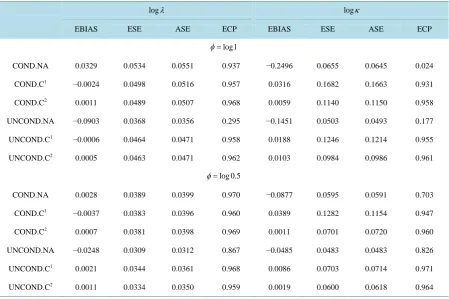
φ is known or unknown, the “correct” likelihood approach reduces the bias of estimates, and the resulting empirical coverage probabilities are all within the acceptable range. These simulations therefore provide empirical support to the claim that the “correct” likelihood approach adjusts for the measurement error and yields consistent estimators. Notable is the only modest increase in the empirical or average standard errors of parameter estimates when the variance of the measurement error distribution is es-timated, especially for the shape parameter κ . The “correct” likelihood approach also provides a good estima-tor of φ, and the empirical bias of estimator for φ is small at 0.03 with standard error 0.27 for the conditional analysis and 0.01 with standard error 0.11 for the unconditional analysis, when φ=log1 0= , for example.

5. Discussion

Statistical models and methods for the analysis of prevalent cohort data have been reviewed here from both the conditional and unconditional frameworks. It is well known that naive analyses which ignore the selection bias lead to overestimation of the survivor probabilities. The conditional likelihood based on the density for left- truncated event times can be used to correct for this selection bias. The unconditional likelihood approach is based on the joint density of the backwards and forward recurrence times yield more efficient estimators by in-corporating the information contained in the onset times. The typical assumption required to formulate the asso-ciated model is of a stationary disease incidence process. Since both approaches make use of the onset time in-formation to correct for selection effects, misspecification of the retrospectively reported disease onset time can have serious implications on the estimation. We investigate the impact of measurement error in disease onset time for prevalent cohort sample and propose “correct” conditional and unconditional likelihoods to account for the measurement error.

[image:10.595.200.429.490.673.2]

The methods we proposed to correct for measurement error in this paper are based on the parametric model. It

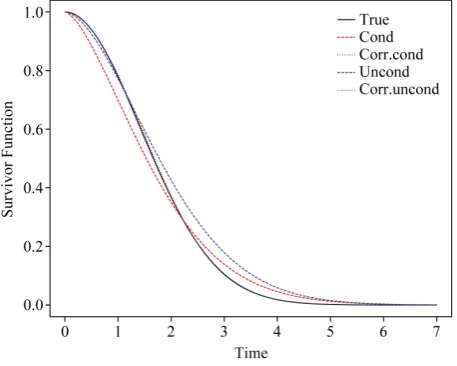
Figure 3. Comparison of the true survivor function with es-timated survivor functions based on conditional likelihood and “correct” conditional likelihood approach; σ = 1, n = 500,

[image:11.595.89.539.121.420.2]

Table 4. Empirical properties of estimators based on the naive conditional likelihood (COND.NA), the corrected condition-al likelihood (COND.C), the naive unconditioncondition-al likelihood (UNCOND.NA), and the corrected unconditioncondition-al likelihood (UNCOND.C); n = 500, nsim = 1000.

logλ logκ

EBIAS ESE ASE ECP EBIAS ESE ASE ECP

log1

φ=

COND.NA 0.0329 0.0534 0.0551 0.937 −0.2496 0.0655 0.0645 0.024

COND.C1 _{−0.0024 0.0498 0.0516 0.957 0.0316 0.1682 0.1663 0.931}

COND.C2 _{0.0011 0.0489 0.0507 0.968 0.0059 0.1140 0.1150 0.958}

UNCOND.NA −0.0903 0.0368 0.0356 0.295 −0.1451 0.0503 0.0493 0.177

UNCOND.C1 −0.0006 0.0464 0.0471 0.958 0.0188 0.1246 0.1214 0.955

UNCOND.C2 _{0.0005 0.0463 0.0471 0.962 0.0103 0.0984 0.0986 0.961}

log 0.5

φ=

COND.NA 0.0028 0.0389 0.0399 0.970 −0.0877 0.0595 0.0591 0.703

COND.C1 _{−0.0037 0.0383 0.0396 0.960 0.0389 0.1282 0.1154 0.947}

COND.C2 _{0.0007 0.0381 0.0398 0.969 0.0011 0.0701 0.0720 0.960}

UNCOND.NA −0.0248 0.0309 0.0312 0.867 −0.0485 0.0483 0.0483 0.826

UNCOND.C1 _{0.0021 0.0344 0.0361 0.968 0.0086 0.0703 0.0714 0.971}

UNCOND.C2 _{0.0011 0.0334 0.0350 0.959 0.0019 0.0600 0.0618 0.964}

1

Denotes case of unknown φ; 2Denotes case of known φ.

is of interest to investigate what the limiting value is of standard nonparametric estimators for both the condi-tional and uncondicondi-tional frameworks. The modest increase in the standard error of the Weibull shape and scale parameters when φ is estimated, suggests that it is promising to consider nonparametric estimation in the cor-rected conditional and unconditional settings. Extending the corcor-rected likelihoods to accommodate misspecifica-tion of the onset times is also of interest for both frameworks.

We focused on the classical error model in this study, but other measurement error models are also of interest; often individuals will report later onset times since their views on disease onset may be more closely tied to the onset of symptoms than the actual disease. Methods to correct for this kind of measurement error are also im-portant and are under development.

References

[1] Zelen, M. and Feinleib, M. (1969) On the Theory of Screening for Chronic Diseases. Biometrika, 56, 601-614.

http://dx.doi.org/10.1093/biomet/56.3.601

[2] Zelen, M. (2004) Forward and Backward Recurrence Times and Length Biased Sampling: Age Specific Models. Life-time Data Analysis, 10, 325-334. http://dx.doi.org/10.1007/s10985-004-4770-1

[3] Lagakos, S.W., Barraj, L.M. and De Gruttola, V. (2006) Nonparametric Analysis of Truncated Survival Data, with Applications to AIDS. Biometrika, 75, 515-523. http://dx.doi.org/10.1093/biomet/75.3.515

[4] Wolfson, C., Wolfson, D.B., Asgharian, M., M’Lan, C.E., Østbye, T., Rockwood, K. and Hogan, D.B. (2001) A Ree-valuation of the Duration of Survival after the Onset of Dementia. New England Journal of Medicine, 344, 1111-1116.

http://dx.doi.org/10.1056/NEJM200104123441501

[5] Asgharian, M., M’Lan, C.E. and Wolfson, D.B. (2002) Length-Biased Sampling with Right Censoring: An Uncondi-tional Approach. Journal of the American Statistical Association, 97, 201-209.

[6] Rothman, K.J., Greenland, S. and Lash, T.L. (2008) Modern Epidemiology. Lippincott Williams & Wilkins, Philadel-phia.

[7] Cox, D.R. and Miller, H.D. (1965) The Theory of Stochastic Processes. Chapman, London.

[8] Kalbfleisch, J.D. and Lawless, J.F. (1991) Regression Models for Right Truncated Data with Applications to AIDS in-cubation Times and Reporting Lags. Statistica Sinica, 1, 19-32.

[9] Turnbull, B.W. (1976) The Empirical Distribution Function with Arbitrarily Grouped, Censored and Truncated Data.

Journal of the Royal Statistical Society, Series B (Methodological), 38, 290-295.

[10] Wang, M.-C. (1991) Nonparametric Estimation from Cross-Sectional Survival Data. Journal of the American Statistic-al Association, 86, 130-143. http://dx.doi.org/10.1080/01621459.1991.10475011

[11] Keiding, N. and Moeschberger, M. (1992) Independent Delayed Entry, Survival Analysis: State of the Art. Springer, New York, 309-326. http://dx.doi.org/10.1007/978-94-015-7983-4_18

[12] Wang, M.-C., Brookmeyer, R. and Jewell, N.P. (1993) Statistical Models for Prevalent Cohort Data. Biometrics, 49, 1-11. http://dx.doi.org/10.2307/2532597

[13] Vardi, Y. (1982) Nonparametric Estimation in the Presence of Length Bias. The Annals of Statistics, 10, 616-620.

http://dx.doi.org/10.1214/aos/1176345802

[14] Vardi, Y. (1989) Multiplicative Censoring, Renewal Processes, Deconvolution and Decreasing Density: Nonparametric Estimation. Biometrika, 76, 751-761. http://dx.doi.org/10.1093/biomet/76.4.751

[15] Vardi, Y. and Zhang, C.-H. (1992) Large Sample Study of Empirical Distributions in a Random-Multiplicative Cen-soring Model. The Annals of Statistics, 20, 1022-1039. http://dx.doi.org/10.1214/aos/1176348668

[16] Asgharian, M. and Wolfson, D.B. (2005) Asymptotic Behavior of the Unconditional NPMLE of the Length-Biased Survivor Function from Right Censored Prevalent Cohort Data. The Annals of Statistics, 33, 2109-2131.

http://dx.doi.org/10.1214/009053605000000372

[17] Huang, C.-Y. and Qin, J. (2011) Nonparametric Estimation for Length-Biased and Right-Censored Data. Biometrika,

98, 177-186. http://dx.doi.org/10.1093/biomet/asq069

[18] Wang, M.-C. (1996) Hazards Regression Analysis for Length-Biased Data. Biometrika, 83, 343-354.

http://dx.doi.org/10.1093/biomet/83.2.343

[19] Luo, X.D. and Tsai, W.Y. (2009) Nonparametric Estimation for Right-Censored Length-Biased Data: A Pseudo-Partial Likelihood Approach. Biometrika, 96, 873-886. http://dx.doi.org/10.1093/biomet/asp064

[20] Tsai, W.Y. (2009) Pseudo-Partial Likelihood for Proportional Hazards Models with Biased-Sampling Data. Biometrika,

96, 601-615. http://dx.doi.org/10.1093/biomet/asp026

[21] Shen, Y., Ning, J. and Qin, J. (2009) Analyzing Length-Biased Data with Semiparametric Transformation and Accele-rated Failure Time Models. Journal of the American Statistical Association, 104, 1192-1202.

http://dx.doi.org/10.1198/jasa.2009.tm08614

[22] Qin, J. and Shen, Y. (2010) Statistical Methods for Analyzing Right-Censored Length-Biased Data under Cox Model.

Biometrics, 66, 382-392. http://dx.doi.org/10.1111/j.1541-0420.2009.01287.x

[23] Wang, M.-C., Jewell, N.P. and Tsai, W.-Y. (1986) Asymptotic Properties of the Product Limit Estimate under Random Truncation. The Annals of Statistics, 14, 1597-1605. http://dx.doi.org/10.1214/aos/1176350180

[24] Qin, J., Ning, J., Liu, H. and Shen, Y. (2011) Maximum Likelihood Estimations and EM Algorithms with Length- Biased Data. Journal of the American Statistical Association, 106, 1434-1449.

http://dx.doi.org/10.1198/jasa.2011.tm10156