An Interactive Method for Two plants Production Inventory Control with Two Warehouse Facility under Imprecise Environment

Volume 96 - No. 21, June 2014

An Interactive Method for Two-plants Production

Inventory Control with Two-warehouse Facility under

Imprecise Environment

Samar Hazari

1

Dept of Mathematics, NIT, Durgapur-713209,

West Bengal, India.

∗

_{Jayanta kumar Dey}

2

Dept of Mathematics, Mahisadal Raj College-721628,

West Bengal, India.

K. Maity

3

Dept of Mathematics, Mugberia Gangadhar Maha-vidyalaya-721425, West Bengal.

Samarjit Kar

1

Dept of Mathematics, NIT, Durgapur-713209,

West Bengal, India.

ABSTRACT

This paper develops an integrated production inventory model with an aim to minimize the cost of production per unit of the product and maximization of profit without compromising the quality of the product. In this model we consider two plants, two secondary warehouses (SWs) and two showrooms (SRs) those are adjacent to the respective plants. For the purpose, we assume to be erected by a firm two plants: Plant-I and Plant-II. Plant-I is situated in an urban area with a lower production capacity in comparison to its product demand where the demand meets through SR-I. On the other hand, Plant-II is situated in a rural area with higher production capacity in comparison to its product demand where the demand meets through SR-II. The excess production in Plant-II meets the current market demand in the area of Plant-I. Here, demand is assumed to be stock dependent in both the showrooms (SR-I and SR-II). Average profit in the integrated model is calculated and global optimum is ob-tained through a descriptive-cum-analytical review. The inventory parameters are taken as fuzzy numbers. The fuzzy numbers are first transformed into corresponding interval numbers and then follow the interval mathematics, the objective function for average profit is converted into respective multi-objective functions. Furthermore, the objective functions are being maximized and solved for a Pareto-optimum solution by interactive fuzzy decision-making pro-cedure. The model also illustrates graphically and numerically.

General Terms:

Two-plants, Two-warehouse,

Keywords:

Inventory, Two-plants, Two-warehouse, Stock dependent demand, Fuzzy inventory cost parameters, Interactive decision making method.

1. INTRODUCTION

The works of Urban[34], Pal et.al.[30], Giri et.al.[11], Padmanab-han and Vrat [28], Sarkar et al[32], Giri and Chaudhuri[12] and others were developed for a single warehouse under the basic as-sumption that the available warehouse has unlimited storage capac-ity. However, this assumption is not realistic. Any warehouse has

Volume 96 - No. 21, June 2014 model with multiple storage facilities where both owned and rented

warehouses had limited stock capacity. Liang and Zhou[23] inves-tigated a two-warehouse inventory model for deteriorating items under conditionally permissible delay in payments. They assumed the rented warehouse had higher unit holding costs than the own warehouse but offered better preservation resulting in a lower rate of deterioration for the goods than in the own warehouse. In reality there are many situations in business sector where the demand rate is not constant but varies. It may depend on time, initial or on hand inventory levels, selling price, advertisement expenditure, the frequency of advertisement etc. There are certain types of items (like consumer goods, fashionable items etc.) for which, according to market research, customers are motivated by the display of the items in the showrooms i.e., the demand rate is dependent on the displayed inventory level. For these items, the consumption goes up if the inventory level is high and vice versa. Many researchers like Levin et al.[22] have observed that the presence of greater quantity of the same item tends to attract more customers. This implies that holding higher inventory level will probably make the retailer sell more items. Under this situation, the demand rate should depend on the inventory level. Such type of demand was considered by Urban[34], Gupta and Vrat[15], Mondal and Phaujdar [25,26], Urban [34,35], Bhuina and Maiti[4] etc. Zhou and Yang[38] presented a two-warehouse inventory model with stock-level-dependent demand rate.

In this study, we considered a production inventory model of two production plants (plant-I and plant-II), two secondary warehouses (SW-I and SW-II) and two showroom-cum-retail outlets (SR-I and SR-II). Production plant-I is situated in an urban area where the density of population is considerably high and thereby there is a high market demand of the product produced in plant-I. The cost of the factors of production in plant-I viz., raw-materials, labour, power, water supply, rent of the factory building etc. is very high and thereby the cost of the production per unit of the output is also very high. In this plant, the rate of production is less in comparison to the market demand of the output produced in plant-I. The plant-I has been erected in the area concerned, where there is a scarcity of the factors of production albeit the locational and other advan-tages for industrial output are prevalent in the area concerned. In order to minimize the total cost of production per unit of the output produced in both the plants and at the same time to meet the high market demand of the product exits in the area of plant-I, another plant-II has been erected in a rural area where the factors of pro-duction required in plant-I is less costly albeit the market demand of the output in the area of plant-II is less than that of the market demand in the area of plant-I. So, the cost of production per unit of output produced in Plant-II is less than that of the cost of produc-tion per unit of output produced in plant-I. It is menproduc-tioned here that the quality standard of the products produced in both the plants are maintained.

There is a large volume of literature on the ’two warehouse inven-tory model’. The literature suggests that the holding cost of sec-ondary warehouse per unit is more than that of the holding cost per unit of showroom cum-outlet. Furthermore, the literature sug-gests that the holding cost per unit in the secondary warehouse is high due to the preservation cost for maintaining the quality of the product and other costs related to handling large quantity of the product in the secondary warehouse. In the present model it is presumed that the holding cost of secondary warehouses is less than the holding cost of showrooms cum-outlets inasmuch as the nature of the output/product produced in both the plants are non-deteriorating and without having any preservation cost. But it is

important to mention here that both the secondary warehouses are located adjacent to the corresponding showroom-cum-retail out-lets and the transportation cost from both the warehouses to show-rooms is insignificant, and hence avoided. Furthermore, the product stored in SW-II is transferred to SW-I through bulk-release-pattern and corresponding transportation cost between two warehouses has been taken into account in the model. This apart, output trans-ferred from both the plants to the showrooms-cum-retail outlets in a continuous-release-pattern. The customer service made from the both the showrooms and the products of both the plants trans-formed on a regular basis / constantly from both the warehouses to both the showrooms to fulfil the demand (as the demand of the product is stock-dependent) even though the holding cost per unit is higher than in showrooms than that of warehouses.

Average profit of the integrated model has been calculated and global optimum was obtained analytically. Here inventory cost pa-rameters are taken imprecise i.e, fuzzy in nature. The said parame-ters are expressed by fuzzy numbers, Which are then converted into appropriate interval numbers following Grzegorzewski[14] and us-ing the concepts of interval arithmetic, we have constructed an equivalent multi-objective deterministic model corresponding to the original problem. This equivalent problem has been solved by using interactive fuzzy decision making procedure. The Opti-mum and Pareto-optiOpti-mum solutions are derived by using a gradient non-linear optimization technique-Generalized Reduced Gradient (GRG) method.

2. THE NEAREST INTERVAL APPROXIMATION

OF A FUZZY NUMBER

According to Grzegorzewski[14], the nearest interval approxi-mation of a Triangular fuzzy number(TFN) A˜ = (a1, a2, a3)

is (a1+a2

2 ,

a2+a3

2 ) and the nearest interval approximation

of a Parabolic fuzzy number(PFN) A˜ = (a1, a2, a3) is

(2a1+a2

3 ,

a2+2a3

3 ).

3. ASSUMPTIONS AND NOTATIONS

Following are the assumptions and notations to develope the model:

3.1 Assumptions

(i) Model is developed for single item product. (ii) Lead time is negligible.

(iii) Demand of customers in the showrooms SR-I and SR-II is stock dependent.

(iv) Shortage are allowed only in SR-I. (v) Idle costs are taken into account.

(vi) Production capacities of two plants are different.

3.2 Notations

q1s(t) = Inventory level of SR-I at time t.

q1r(t) = Inventory level of SW-I at time t.

q2s(t) = Inventory level of SR-II at time t. q2r(t) = Inventory level of SW-II at time t.

P1 = Constant production rate of plant-I

(P1< a1, a1>0).

P2 = Constant production rate of plant-II.

Volume 96 - No. 21, June 2014 W2 = Capacity of SR-II.

D1(t) = Demand rate of SR-I,where

D1(t) =

(_a

1 when0≤t < t1

a1+b1W1 whent1≤t < t2+k

0

a1+b1q1s(t) whent2+k

0

≤t≤Tp₁ a1, b1 are constant.

D2(t) = Demand rate of SR-II, where

D2(t) =

(

a2 when0≤t < t

0

1

a2+b2W2 whent

0

1≤t < t3

a2+b2q2s(t) whent3≤t≤Tp2

a2, b2 are constant.

S1 = Shortage amount in SR-I at timet1.

c1s = Shortage cost per unit per unit time in SR-I of plant-I. h1s = Holding cost per unit per unit time of SR-I.

h1r = Holding cost per unit per unit time of SW-I. h2s = Holding cost per unit per unit time of SR-II. h2r = Holding cost per unit per unit time of SW-II. cp₁ = Production cost per unit item for plant-I. cp2 = Production cost per unit item for plant-II.

s1 = Selling price per unit item in SR-I.

s2 = Selling price per unit item in SR-II.

p0₁ = Transfer rate of produce items from SW-I to SR-I during (t1, tp1).

p00₁ = Transfer rate of produce items from SW-I to SR-I during (tp1, t2+k

0

).

k = Time duration of shifting the amountkp01from SW-II to SW-I

during(t1, tp1).

k0 = Time duration of shifting the amountk0p001from SW-II to SW-I

during(tp₁, t2).

t1 = Time where SR-I received of amount(S1+W1).

tp₁ = Time where plant-I stop its production. tp₂ = Time where plant-II stop its production. Tp₁ = Time where items are exhausted from SR-I. Tp₂ = Time where items are exhausted from SR-II. t2 = Time of shifting last lot from SW-II to SW-I.

t3 = Time where items are exhausted from SW-II.

A1s = Ordering cost for SR-I. A2s = Ordering cost for SR-II. A1r = Ordering cost for SW-I. A2r = Ordering cost for SW-II. id1s = Idle cost per unit time of SR-I. id2s = Idle cost per unit time of SR-II. id1r = Idle cost per unit time of SW-I. id2r = Idle cost per unit time of SW-II.

n = Number of times to shifting the amountp0₁kin each time from SW-II to SW-I during[t1, tp1].

r = Number of times to shifting the amountp001k

0

in each time from SW-II to SW-I during[tp1, tp2].

m−r = Number of times to shifting the amountp001k

0

in each time from SW-II to SW-I during[tp₂, t2].

4. MODEL DESCRIPTION AND DIAGRAMMATIC

REPRESENTATION

The production plants (i.e plant-I and plant-II), starts their produc-tion at timet= 0and produced items are selling through the show-rooms(i.e SR-I and SR-II). In plant-I, the production rate is lower than the demand rate of SR-I and thus shortages occurs at SR-I for time period(0, t1). In plant-II, the production rate is higher than

demand rate of SR-II, so excess items are stored in the secondary ware house SW-II at the rateP2−D2in continuous release pattern.

At timet1, for one time, the items of amount(S1+W1+kp

0

1)are

transferred from SW-II to fulfill the shortage amountsS1at SR-I,

to filled up the showroom SR-I by the amountW1and rest amount

kp01 is stored in the secondary ware house SW-I. Items are then

transferred from SW-I to SR-I in continuous release pattern at the ratesp0₁andp00₁during the period(t1, tp1)and(tp1, t2+k

0

) respec-tively to filled-up showroom SR-I continuously, as the demand rate at SR-I is stock depended. The items are transferred from SW-II to SW-I in bulk release pattern of amountkp01with time intervalk

and of amountk0p001with time intervalk

0

for n and m times during the periods(t1, tp1)and(tp1, t2)respectively. The amountkp

0

1is

transferred r times among m times with time intervalk0for the pe-riod(tp1, tp2). As demand is stock dependent at SR-II, so the items

are continuously transferred with rateD2to filled-up the showroom

SR-II from the production plant-II and SW-II during(0, tp₂)and (tp₂, t3)respectively.

[image:3.595.320.554.434.611.2]

Mathematical formulation for different showrooms and secondary warehouses are depicted in different sub-section. The block dia-grams of production inventory model is given in Fig.-1.

Volume 96 - No. 21, June 2014

5. MATHEMATICAL FORMULATION OF THE

MODEL

5.1 For Showroom-I(SR-I)

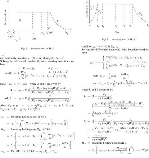
Differential equation for the SR-I in[0, Tp₁]is given by

dq1s

dt =

 



P1−a1, 0≤t < t1

0, t1≤t < t2+k

0

−[a1+b1q1s(t)], t2+k

0

≤t≤Tp₁ (1)

[image:4.595.53.534.200.708.2]

with boundary conditionq1s(t) = 0att= 0, Tp1,q1s(t1−0) =

Fig. 2. Inventory level of SR-I

−S1

and continuity conditionq1s(t) =W1during[t1, t2+k

0

]. Solving the differential equation (1) with boundary conditions, we have

q1s(t) =

 



(P1−a1)t, 0≤t < t1

W1, t1≤t < t2+k

0

a1

b1

eb1(Tp1−t)−_{1, t2+k}0 ≤_t≤_Tp 1

Here S1 = A+Bk where A and B are given by

A = (a1−P1)

t 0

1(P2−(a2+b2W2)) +W1

(P2−(a2+b2W2))−(a1−P1)

and, B = (a1−P1)

P

0

1

(P2−(a2+b2W2))−(a1−P1)

Also, P1 + p

0

1 = a1 + b1W1, p

00

1 = a1 + b1W1 and

Tp₁ =t2+k

0

+ 1

b1log(1 +

b1W1

a1 )

S1s = Inventory Shortage cost of SR-I

= c1s

−

Z t1

0

(P1−a1)tdt

=−c1s

(P1−a1)

t2 1

2

H1s = Inventory holding costH1sof SR-I

= h1s

W1(t2+k

0

−t1) +

Z Tp1

t2+k0

a1

b1

eb1(Tp1−t)−_1dt

= h1s

W1(t2+k

0

−t1) +

W1

b1

−a1

b2 1

log(1 +b1W1 a1

)

Id1s = The idle cost of SR-I =id1s(Tp2−Tp1)

5.2 For Showroom-II (SR-II)

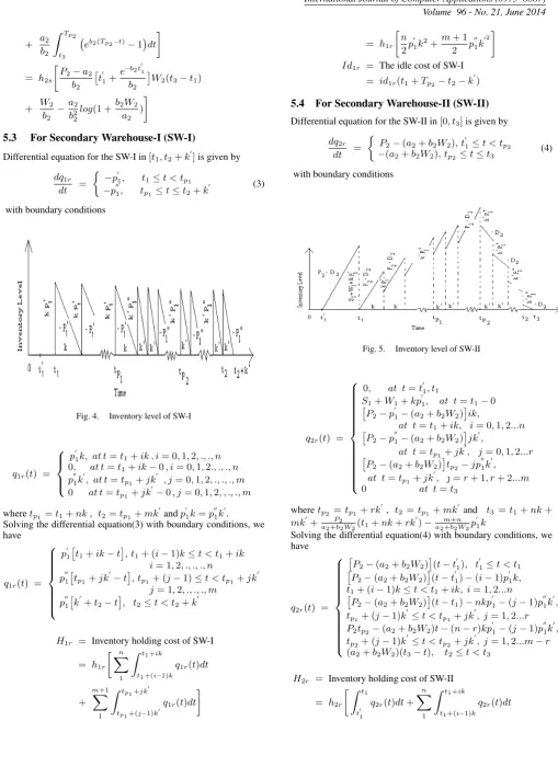
Differential equation for the SR-II in[0, Tp2]is given by

dq2s

dt =

( _P

2−(a2+b2+W2q2s(t)),0≤t < t

0

1

0, t0₁≤t < t3

−(a2+b2+W2q2s(t)), t3≤t≤Tp2

(2)

[image:4.595.70.285.200.341.2]

with boundary conditionq2s(t) = 0,att= 0, Tp2, and continuity

Fig. 3. Inventory level of SR-II

conditionq2s(t) =W2in[t

0

1, t3].

Solving the differential equation(2) with boundary conditions, we have

q2s(t) =

  

 

(P2−a2)

b2 (1−e

−b2t_{), 0≤t < t}0 1

W2, t

0

1≤t < t3

a2

b2

eb2(Tp2−t)−_{1, t3}≤_t≤_Tp 2

with t01=−

1 b2

log(1−b2W2

a2

)

and,Tp2=t3+

1 b2

log(1 +b2W2 a2

) =U+V k

where U and V are given by

U = (1 + P2 a2+b2W2

)

(a1−P1)

t0₁(P2−(a2+b2W2))+W1

(P2−(a2+b2W2))−(a1−P1)

+W1

P2−a2−b2W2

+ 1

b2

log(1 +b2W2 a2

)>0

V = (1 + P2 a2+b2W2

) p

0

1

(P2−a2−b2W2)−(a1−P1)

+ n(P2+a2+b2W2 a2+b2W2

) +m(a2+b2W2) +rP2 a2+b2W2

p0₁ p00₁

− m+n

a2+b2W2

p001

H2s = Inventory holding cost of SR-II

= h2s

W1(t3−t1) +

(P2−a2)

b2

Z t 0

1

0

Volume 96 - No. 21, June 2014

+ a2 b2

Z Tp2

t3

eb2(Tp2−t)−_1dt

= h2s

P2−a2

b2

t0₁+e

−b2t

0

1

b2

W2(t3−t1)

+ W2 b2

−a2

b2 2

log(1 +b2W2 a2

)

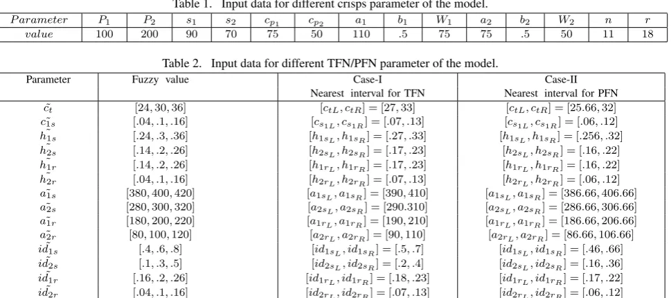
5.3 For Secondary Warehouse-I (SW-I)

Differential equation for the SW-I in[t1, t2+k

0

]is given by

dq1r

dt =

−p01, t1≤t < tp1

−p00₁, tp₁ ≤t≤t2+k

0 (3)

with boundary conditions

Fig. 4. Inventory level of SW-I

q1r(t) =   

 

p01k, at t=t1+ik , i= 0,1,2, ., ., n

0, at t=t1+ik−0, i= 0,1,2., ., ., n

p00₁k0, at t=tp1+jk

0

, j= 0,1,2, ., ., ., m 0 at t=tp₁+jk0−0, j= 0,1,2, , ., ., m wheretp₁=t1+nk, t2=tp1+mk

0

andp01k=p

00

1k

0 . Solving the differential equation(3) with boundary conditions, we have

q1r(t) =       

     

p01

t1+ik−t

, t1+ (i−1)k≤t < t1+ik

i= 1,2, ., ., ., n

p00₁tp₁+jk0−t, tp₁+ (j−1)≤t < tp₁+jk0 j= 1,2, ., ., ., m

p001

k0+t2−t

, t2≤t < t2+k

0

H1r = Inventory holding cost of SW-I

= h1r n

X

1

Z t1+ik

t1+(i−1)k q1r(t)dt

+ m+1

X

1

Z tp₁+jk0 tp1+(j−1)k

0

q1r(t)dt

= h1r

n 2p

0

1k

2₊m+ 1

2 p

00

1k

02

Id1r = The idle cost of SW-I

= id1r(t1+Tp2−t2−k

0

)

5.4 For Secondary Warehouse-II (SW-II)

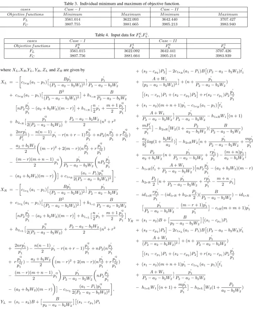
Differential equation for the SW-II in[0, t3]is given by

dq2r

dt =

P2−(a2+b2W2), t

0

1≤t < tp2

−(a2+b2W2), tp2≤t≤t3

(4)

[image:5.595.51.561.39.739.2]

with boundary conditions

Fig. 5. Inventory level of SW-II

q2r(t) =             

           

0, at t=t01, t1

S1+W1+kp

0

1, at t=t1−0

P2−p

0

1−(a2+b2W2)

ik,

at t=t1+ik, i= 0,1,2...n

P2−p

00

1−(a2+b2W2)

jk0,

at t=tp₁+jk0, j= 0,1,2...r

P2−(a2+b2W2)

tp2−jp

00

1k

0

, at t=tp₁+jk0,  =r+ 1, r+ 2...m

0 at t=t3

wheretp₂ =tp₁+rk0 , t2 =tp1+mk

0

and t3 =t1+nk+

mk0+ P2

a2+b2W2(t1+nk+rk

0

)− m+n a2+b2W2p

0

1k

Solving the differential equation(4) with boundary conditions, we have

q2r(t) =

          

         

P2−(a2+b2W2)

(t−t0₁), t0₁≤t < t1

P2−(a2+b2W2)

(t−t01)−(i−1)p

0

1k,

t1+ (i−1)k≤t < t1+ik, i= 1,2...n

P2−(a2+b2W2)

(t−t1)−nkp

0

1−(j−1)p

00

1k

0

, tp₁+ (j−1)k0≤t < tp₁+jk0, j= 1,2...r P2tp2−(a2+b2W2)t−(n−r)kp

0

1−(j−1)p

00

1k

0

, tp₂+ (j−1)k0≤t < tp₂+jk0, j= 1,2...m−r (a2+b2W2)(t3−t), t2≤t < t3

H2r = Inventory holding cost of SW-II

= h2r Z t1

t0₁

q2r(t)dt+ n X

1

Z t1+ik

t1+(i−1)k

Volume 96 - No. 21, June 2014

+ r X

1

Z tp1+jk

0

tp₁+(j−1)k0

q2r(t)dt+

m−r X

1

Z tp2+jk

0

tp₂+(j−1)k0

q2r(t)dt

+ Z t3

t2

q2r(t)dt

= h2r

P2−(a2−b2W2)

2 (t1−t

0

1)

2

+ P2−(a2−b2W2)

2 n

2_k2₋n(n+ 1)

2 p

0

1k2

+ P2−(a2−b2W2) 2

2nrkk0+r2_k02

−nrp00₁k02

− r(r+ 1)

2 p

00

1k

02

+nP2(t1+nk+rk

0

)k0

− (a2−b2W2)

2

(m−r)2_k2_{+ 2(m−r)(t}

1+nk+rk

0

)k0

− (m−r)(m+n−1)

2 p

0

1k2+

(a2−b2W2)

2 (t2−t3)

2

Id2r = The idle cost of SW-II=id2r(Tp2−t3)

Ct = total transportation cost

= ct[S1+W1+ (m+n+ 1)kp

0

1]

6. INTEGRATED MODEL:

6.1 In Crisp Environment

Total profit of the production inventory systemT Pis given by

T P = Total profit of the production inventory system = Revenue from sales -production cost -S1s-H1s-H2s

-H1r-H2r-Id1s-Id2s-Id1r-Id2r-Ct-A1s-A2s-A1r-A2r = Xk2+Y k+Zwhere X , Y and Z are given by

X = −

c1s(a1−p1)

Bp

0

1

(P2−a2−b2W2)2

p

0

1

P2−a2−b2W2

+ c1s(a1−p1)

B2

(P2−a2−b2W2)2

+h1r

B P2−a2−b2W2

nP2

p0₁

p00₁ −(a2+b2W2)(m−r)

+h1r n

2p

0

1+

m+ 1 2

p0₁2 p00₁

+ h2r

p

02 1

2(P2−a2−b2W2)

+P2−a2−b2W2

2 (n

2

+r2

+ 2nrp

0

1

p0₁ )−

n(n−1)

2 p

0

1−r(n+r−1)

p0₁2

p00₁ +nP2(n p0₁ p00₁

+ rp

02 1

p0012

)−a2+b2W2

2

(m−r)2+ 2(m−r)(np

0

1

p00₁ +r p012

p0012

)

− (m−r)(m+n−1)

2 p

02 1

p01

P2−a2−b2W2

nP2

p01

p00₁

− (a2+b2W2)(m−r)

+cs₁ (a1−P1)p

02 1

2(P2−a2−b2W2)2

<0,

Y = (s1−s2)B+

B

P2−a2−b2W2

(s1−cp1)P1+ (s2−cp2)P2

− 2c1s(a1−P1)B

(P2−a2−b2W2)t

0

1

+ A+W1

(P2−a2−b2W2)2

+ (n+ p

0

1

P2−a2−b2W2

)

(s1−cp1)P1+ (s2−cp2)P2

+r(s2−cp1)

P2

p01

p001

+ (s1−s2)(m+n+ 1)p

0

1

− cs1(a1−p1)

t01+

A+W1

P2−a2−b2W2

p0₁ P2−a2−b2W2

−h1sW1

(n+ 1) +mp

0

1

p00₁

− h2s

W2(1 +

P2

a2−b2W2

)( B

P2−a2−b2W2

)

− a2

b2 2

log(1 +b2W2 a2

)−h2sW2

n

+ p

0

1

P2−a2−b2W2

+mp

0

1

p00₁ + P2

a2+b2W2

(n+ p

0

1

P2−a2−b2W2

+rp

0

1

p00₁ )−

(m+n)p01

a2−b2W2

− h1r(t

0

1+

A+W1

P2−a2−b2W2

)nP2

p01

p00₁ −(a2+b2W2) (m−r)−h2r

P2

2

n+ p

0

1

P2−a2−b2W2

+rp

0

1

p00₁

− m+n

2 p

0

1

−id1s rp01

p00₁ −(id1r+h2r P2

2 )

( B

P2−a2−b2W2

)−id1r

p

0

1

P2−a2−b2W2

− (m−r+ 1)p

0

1

p001

−ct(m+m+ 1)p

0

1

and, Z = (s1−s2)(A+W1) +

t01+

A+W1

P2−a2−b2W2

(s1−cp1)P1+ (s2−cp2)P2

−c1s(a1−P1)

t01+

A+W1

P2−a2−b2W2

2

−c1s(a1−P1)

(P2−a2−b2W2)t

0

1+A+W1

P2−a2−b2W2

2

− h1s W1

b1

−a1

b2 1

log(1 +b1W1 a1

)

− h2s

P2−a2

b2

(t0₁+ 1 b2

P2−a2−b2W2

P2−a2

)

+ W2(1 +

P2

a2−b2W2

)(t01+

A+W1

P2−a2−b2W2

)

− a2

b2 2

log(1 +b2W2 a2

)−(id1r+h2r P2

2 )

(t01+

A+W1

P2−a2−b2W2

)−id2r 1

b2

log(1 +b2W2 a2

)

Volume 96 - No. 21, June 2014 The average profit ATP(k) is given by

AT P(k) = T P Tp2

=Xk

2_{+Y k+Z}

U+V k (5)

For optimum value of ATP(k),we must have

d(AT P)

dk = 0

⇒ V Xk2+ 2U Xk+ (U Y −V Z) = 0

⇒ k=−U

V ±

r U2

V2 −

U Y −V Z V X

Now d

2_{(AT P)}

dk2

k=k∗

<0

for U2X−V(U Y −V Z)<0

and U Y −V Z >0 (6)

Wherek∗

is the corresponding optimal value of k and given by

k∗=−U

V +

r U2

V2 −

U Y −V Z

V X (7)

Therefore ATP is concave fork = k∗ _{if the inequations in (6)}

holds. Substituting the value ofk∗_{in (5) we get the optimum value}

AT P∗(k)ofAT P(k).

6.2 In Fuzzy Environment

Considering all holding costs, shortage costs, set-up costs, and transportation cost as fuzzy numbers and then from equation (5), average total profit of the system is given by

˜

AT P(k) = T P Tp₂ =

˜

Xk2_{+ ˜Y k+ ˜Y}

U+V k (8)

whereX˜,Y˜andZ˜are given by

˜

X = −

˜

c1s(a1−p1)

Bp

0

1

(P2−a2−b2W2)2

p

0

1

P2−a2−b2W2

+ c˜1s(a1−p1)

B2

(P2−a2−b2W2)2

+ ˜h1r

B P2−a2−b2W2

nP2

p01

p001

−(a2+b2W2)(m−r)

+ ˜h1r

n 2p

0

1+

m+ 1 2

p012

p001

+ h˜2r

p

02 1

2(P2−a2−b2W2)

+P2−a2−b2W2

2 (n

2_+r2

+ 2nrp

0

1

p0₁ )−

n(n−1)

2 p

0

1−r(n+r−1)

p012

p00₁ +nP2(n p01

p00₁

+ rp

02 1

p00₁2)−

a2+b2W2

2

(m−r)2+ 2(m−r)(np

0

1

p001

+rp

02 1

p00₁2)

− (m−r)(m+n−1)

2 p

02 1

p01

P2−a2−b2W2

nP2

p01

p00₁

− (a2+b2W2)(m−r)

+ ˜c1s

(a1−P1)p

02 1

2(P2−a2−b2W2)2

,

˜

Y = (s1−s2)B+

B

P2−a2−b2W2

(s1−cp1)P1

+ (s2−cp2)P2

−2 ˜c1s(a1−P1)B

(P2−a2−b2W2)t

0

1

+ A+W1

(P2−a2−b2W2)2

+ (n+ p

0

1

P2−a2−b2W2

)(s1−cp1)P1

+ (s2−cp2)P2

+r(s2−cp1)P2

p01

p00₁ + (s1−s2) (m+n+ 1)p0₁−c˜1s(a1−p1)

t0₁

+ A+W1

P2−a2−b2W2

p

0

1

P2−a2−b2W2

− h˜1sW1

(n+ 1) +mp

0

1

p00₁

−h˜2s

W2(1

+ P2

a2−b2W2

)( B

P2−a2−b2W2

)− a2

b2 2

log(1 +

b2W2

a2

)−h˜2sW2

n+ p

0

1

P2−a2−b2W2

+mp

0

1

p00₁

+ P2

a2+b2W2

(n+ p

0

1

p2−a2−b2W2

+rp

0

1

p00₁ )

− (m+n)p

0

1

a2−b2W2

−h˜1r(t

0

1+

A+W1

P2−a2−b2W2

)

nP2

p01

p001

−(a2+b2W2)(m−r)

−h˜2r P2

2

n+

p01

P2−a2−b2W2

+rp

0

1

P100

− m+n

2 p

0

1

−id˜1s rp01

p001

− ( ˜id1r+ ˜h2r P2

2 )(

B P2−a2−b2W2

)

− _id˜_1r p 0

1

P2−a2−b2W2

−(m−r+ 1)p

0

1

p00₁

− ct(m˜ +m+ 1)p01

and,Z˜ = (s1−s2)(A+W1) +

t0₁+ A+W1 P2−a2−b2W2

(s1−cp1)P1+ (s2−cp2)P2

−c˜1s(a1−P1)

t0₁+ A+W1 P2−a2−b2W2

2

−c˜1s(a1−P1)

(P2−a2−b2W2)t

0

1+A+W1

P2−a2−b2W2

2

− h˜1s W1

b1

− a1

b2 1

log(1 +b1W1 a1

)−h˜2s

P2−a2

b2

(t01+

1 b2

P2−a2−b2W2

P2−a2

) +W2(1 +

P2

a2−b2W2

)(t0₁+ A+W1 P2−a2−b2W2

)

− a2

b2 2

log(1 +b2W2 a2

)−( ˜id1r+ ˜h2r P2

2 )

(t01+

A+W1

P2−a2−b2W2

)−id˜2r 1

b2

log(1 +

b2W2

a2

)−c˜t(A+W1)−A˜1s−A˜2s

− A˜1r−A˜2r

trans-Volume 96 - No. 21, June 2014 formed to interval numbers and the expression (8) is expressed as

˜

AT P(k) = FL, FR (9)

(For detail calculations ofFLandFR, see Appendix-A)

According to Dey et.al[10], the interval problem (9) can be repre-sented as

Maximize{FL, FC} (10)

whereFC= (FL+FR)/2.

7. INTERACTIVE APPROACH

Now considering the imprecise nature of DM’s judgement, DM may have different fuzzy or imprecise goals for each of the ob-jective functions and hence interactive approach is used for the man-machine interaction. To derive the membership functionsµF_L and µF_C for the objective functions FL and FC respectively from DM’s viewpoint, we first calculate individual minimum(i.e. Fmin

L , FCmin) and individual maximum(i.e. FLmax, FCmax) by a non-linear optimization technique. With the help of individual min-imum and maxmin-imum, the DM can select any one from among the following three types of membership functions

(i) Linear membership functions. (ii) Quadratic membership functions. (ii) Exponential membership functions.

The membership functionsµF_LandµF_C for the corresponding ob-jective functionsFLandFCcan be written as

µF_k=

( _{1, if Fk≤F}0

k, dk, if Fk0≤Fk≤F

1

k,

0, if F1

k ≤Fk

(11)

whereF0

kandFk1are to be chosen such thatFkmin≤Fk0≤Fk1≤ Fmax

k anddkis a strictly monotonic decreasing continuous func-tion ofFkwhich may be linear or non-linear.

7.1 Description of the Membership functions

7.1.1 Linear membership function (Type-I). For each objec-tive function, the corresponding Linear membership functions are as follows:

µF_k=   

 

1, if Fk≤F0

k,

1−F

1

k−Fk

Pk , if F

0

k ≤Fk≤F

1

k,

0 if F1

k ≤Fk (12)

whereF0

kandF

1

kare to be chosen such thatF min

k ≤F

0

k ≤F

1

k ≤ Fmax

k andPk=Fk1−Fk0is the tolerance of k-th objective function Fk

7.1.2 Quadratic membership function (Type-II). For each ob-jective function, the corresponding quadratic membership func-tions are as follows:

µF_k=   

 

1, if Fk≤F0

k,

1−

F1

k−Fk Pk

2

,if Fk0≤Fk≤F

1

k,

0, if Fk1≤Fk

(13)

whereF0

kandFk1are to be chosen such thatFkmin≤Fk0≤Fk1≤ Fmax

k andPk=Fk1−Fk0is the tolerance of k-th objective function Fk.

7.2 Fuzzy decision method

After determining the different linear/nnon-linear membership functions(MF) for each of the objective functions, following Bellman and Zadeh[1] and Zimmermannn[36], the given prob-lem(10)can be formulated as

Maximize λ

Subject to λ≤µF_L, λ≤µF_C (14)

0≤λ≤1.

with the help of two different types of membership functions given by (12) and (13),the above problem can be restated for a particular choice of DM as

Maximize λ

Subject to λ≤1− F

1

L−FL

PL ,

if the M F of f irst objective ∈ T ype−I, λ≤1−

F1

C−FC PC

2

, (15)

if the M F of f irst objective ∈ T ype−II, 0≤λ≤1.

Here DM selects the above membership functions for the cor-responding objective functions. Then the above problem can be solved by a non-linear optimization technique and optimal solu-tion ofλ, sayλ∗

is obtained. Now after obtainingλ∗

, the DM selects the most important objec-tive function from among the objecobjec-tive functionsFLandFC. Here FLis selected as DM would like to maximize his/her worst case. Then the problem becomes(λ=λ∗₎

Maximize FL

Subject to FL≥mL, FC≥mC (16) 0≤λ≤1.

Where mL=FL1−(F

1

L−F

0

L)(1−λ

∗

), if the M F of f irst objective ∈ T ype−I, mC=FC1 −(F

1

C−F

0

C)(1−λ

∗

)12_,

if the M F of f irst objective ∈ T ype−II, 0≤λ≤1.

7.3 Pareto-optimal solution

Now, after deriving the optimum decision variables, Pareto-optimality test is performed according to Sakawa[31]. Let the de-cision variablek∗_{and optimum values,F}∗

L=FL(k

∗_)andF∗

C =

FC(k∗_{)are obtained from (16). With these values, the following}

problem is solving using a non-linear optimization technique:

Minimize V = (L+C)

Subject to FL−L=FL∗, FC−C=F

∗

C (17)

L, C≥0, 0≤λ≤1.

Volume 96 - No. 21, June 2014

8. NUMERICAL EXAMPLE

To illustrate the proposed inventory model, following crisp input data are considered in table-1. We consider case-I, when fuzzy pa-rameters are TFN and case-II when fuzzy parameter are PFN.The nearest interval approximation according to Grzegorzewski[14] in both cases(i.e, case-I and case-II)are given in Table-2.

Following (14) and (15), the problem (9) is solved and the results are presented in Table-3 and Table-4.

Let, with the above values, the membership functions of the objec-tive functions be formed of the types as per Table 5.

Let, at the beginning, analysis is performed to find optimumλwith the membership functionsFLas linear(Type-I) andFCas quadratic (Type-II). The optimum value ofλis presented in Table-6. With this value ofλ∗_{, the objective functionFLis optimized and}

the optimum results are given in Table-7.

Now, the results obtained from Table-7 are tested for pareto-optimality and the pareto-optimal results are given in Table-8.

9. DISCUSSION:

In Table 8, the values of V are quite small in both cases and hence, the optimum results in table 7 are strong Pareto-optimum and can be accepted.Still, if the decision-maker/practitioner is not satisfied with the outputs, he/she may perform the above analysis again re-choosing the membership functions forFLand FC as linear, quadratic and exponential(say). If the second time analysis does not also give the desired result, the DM may perform the analysis with the other possible different combinations(in this case,32_{times) of}

the membership functions and can select the most suitable optimum solution for his/her firm/factory for implementation.Furthermore we observed that the average profit is greater in case-II than Case-I.

10. CONCLUSION

This production inventory model, which comprises of two pro-duction plants, two secondary warehouses and two showrooms, is aiming at minimizing the overall production cost per unit of product. In order to attain it we derived a closed form of solution of the model. Here, two plant concepts were used in the sense that a manufacturer / firm wanted to minimize the overall production cost by erecting two plants in two different regions / areas. In a nut shell, the study suggests that the production cost per unit of the product will minimize and thereby the total net profit will maximize by erecting two plants out of which one plant has substantially lower production cost per unit than the other.

Acknowledgements:Dr. Jayanta Kumar Dey thanks the Minor Re-search Project (PSW-138, 09/10 UGC, Govt. of India) for financial support to do this research work.

11. REFERENCE

[1] Bellman, R.E., and Zadeh, L.A; ”Decision-making in a fuzzy environment”, Management Science,Vol. 17, pp. B141-B164,1970.

[2] Benkherouf,L; ” A deterministic order level inventory model for deteriorating items with two storage facilities”, Interna-tional Journal Production Economics,vol. 48, pp. 167-175, 1997.

[3] Bhunia, A. K. and Maiti,M; ” A two warehouse inventory model for a linear trend in demand”, Opsearch, Vol. 31, pp. 318-329, 1994.

[4] Bhunia, A. K. and Maiti, M; ”A deterministic two storage in-ventory model for variable production and inin-ventory level depen-dent demand rate”, Cahiers du CERO, Vol. 37, pp. 17-24, 1995. [5] Bhunia,A. K., and Maiti, M; ” A two warehouses inventory model for deteriorating items with a linear trend in demand and shortages”, Journal of Operational Research Society,Vol. 49,pp. 289-292, 1998.

[6] Chung, K., Her, C., and Lin, S; ” A two-warehouse inventory model with imperfect quality production processes”, Computers and Industrial Engineering, Vol. 56,pp. 193-197, 2009.

[7] Chung, K. and Huang, T;” The optimal retailer’s ordering poli-cies for deteriorating items with limited storage capacity under trade credit financing”. International Journal of Production Eco-nomics, Vol. 106, pp.127-146,2007.

[8] Dave, U; ”On the EOQ models with two levels of storage”, Opsearch, Vol. 25, pp. 190-196,1988.

[9] Dey, J.K., Kar,S., and Maiti,M;” An interactive method for inventory control with fuzzy lead-time and dynamic demand”, European Journal of Operational Research, Vol. 167 ,pp. 381-397,2005.

[10] Dey,J.K.,Mondal,S.K.,and Maiti, M; ” Two storage inven-tory problem with dynamic demand and interval valued lead-time over finite lead-time horizon under inflation and lead-time-value of money”, European Journal of Operational Research, Vol. 185,pp. 170-194, 2008.

[11] Giri,B. C., Pal, S., Goswami, A., and Chaudhuri,K. S; ”An in-ventory model for deteriorating items with stock-dependent de-mand rate”, European Journal of Operational Research,Vol. 95, pp.604-610,1996.

[12] Giri, B. C., and Chaudhuri,K. S;”Deterministic models of per-ishable inventory with stock-dependent demand rate and non-linear holding cost”, European Journal of Operational Research, Vol. 105,pp. 67-474, 1998.

[13] Goswami,A. and Chaudhuri,K.S; ” An economic order quan-tity model for items with two level of storage for a linear trend in demand”, Journal of Operational Research Society,Vol.43, pp. 157-167, 1992.

[14] Grzegorzewski, P; ”Nearest Interval approximation of a Fuzzy Number, Fuzzy Sets and Systems,Vol. 130,pp. 321-330,2002.

[15] Gupta, R. and Vrat P; ” An EOQ model for stock dependent consumption rate”,Opsearch,Vol. 23,pp. 19- 24,1986.

[16] Hariga, M;”Inventory models for multi-warehouse systems under fixed and flexible space leasing contracts”. Computers and Industrial Engineering,Vol. 61,pp. 744-751,2011.

[17] Hartely,R. V;”Operations Research - A Managerial Emphasis, Good Year Publishing Company”, California,pp. 315-317, 1976. [18] Hsieh, T., Dye, C., and Ouyang, L; ”Determining optimal lot size for a two-warehouse system with deterioration and short-ages using net present value”. European Journal of Operational research,Vol. 191, pp. 182-192, 2008.

[19] Kar,S. K., Bhunia, A. K., and Maiti, M; Deterministic inven-tory model with levels of storage, a linear trend in demand and a fixed time horizon, Computer and Operations ResearchVol. 28 , pp. 1315 - 1331, 2001.

[image:10.595.66.551.68.283.2]

Volume 96 - No. 21, June 2014 Table 1. Input data for different crisps parameter of the model.

P arameter P1 P2 s1 s2 cp1 cp2 a1 b1 W1 a2 b2 W2 n r

value 100 200 90 70 75 50 110 .5 75 75 .5 50 11 18

Table 2. Input data for different TFN/PFN parameter of the model.

Parameter Fuzzy value Case-I Case-II

Nearest interval for TFN Nearest interval for PFN

˜

ct [24,30,36] [ctL, ctR] = [27,33] [ctL, ctR] = [25.66,32] ˜

c1s [.04, .1, .16] [cs1L, cs1R] = [.07, .13] [cs1L, cs1R] = [.06, .12] ˜

h1s [.24, .3, .36] [h1sL, h1sR] = [.27, .33] [h1sL, h1sR] = [.256, .32] ˜

h2s [.14, .2, .26] [h2sL, h2sR] = [.17, .23] [h2sL, h2sR] = [.16, .22] ˜

h1r [.14, .2, .26] [h1rL, h1rR] = [.17, .23] [h1rL, h1rR] = [.16, .22] ˜

h2r [.04, .1, .16] [h2rL, h2rR] = [.07, .13] [h2rL, h2rR] = [.06, .12] ˜

a1s [380,400,420] [a1sL, a1sR] = [390,410] [a1sL, a1sR] = [386.66,406.66] ˜

a2s [280,300,320] [a2sL, a2sR] = [290.310] [a2sL, a2sR] = [286.66,306.66] ˜

a1r [180,200,220] [a1rL, a1rR] = [190,210] [a1rL, a1rR] = [186.66,206.66] ˜

a2r [80,100,120] [a2rL, a2rR] = [90,110] [a2rL, a2rR] = [86.66,106.66] ˜

id1s [.4, .6, .8] [id1sL, id1sR] = [.5, .7] [id1sL, id1sR] = [.46, .66] ˜

id2s [.1, .3, .5] [id2sL, id2sR] = [.2, .4] [id2sL, id2sR] = [.16, .36] ˜

id1r [.16, .2, .26] [id1rL, id1rR] = [.18, .23] [id1rL, id1rR] = [.17, .22] ˜

id2r [.04, .1, .16] [id2rL, id2rR] = [.07, .13] [id2rL, id2rR] = [.06, .12]

[21] Lee, C. and Ma, C;”Optimal inventory policy for dete-riorating items with two-warehouse and time-dependent de-mands”.Production Planning and Control,Vol. 11, pp. 689-696, 2000.

[22] Levin, R. I., Mclaughlin, C. P. , Lamone, R.P. and Kottas, J. F; ”Production / Operations management: contemporary policy for managing operating systems”, McGraw-Hill, New York,pp. 373-387,1972.

[23] Liang, Y. and Zhou, F;”A two-warehouse inventory model for deteriorating items under conditionally permissible delay in payment”. Applied Mathematical Modelling, Vol.35,pp. 2221-2231,2011.

[24] Liao, J. and Huang, K; ”Deterministic inventory model for deteriorating items with trade credit financing and capacity con-straints”. Computers and Industrial Engineering, Vol. 59,pp. 611-618, 2010.

[25] Mandal, B. N. and Phaujder, S; ”An inventory model for de-teriorating items and stock dependent consumption rate”,Journal of Oprational Research Society,Vol. 40, pp. 483 - 488, 1989A. [26] Mandal, B. N. and Phaujder, S;”A note on an inventory model

with stock dependent consumption rate”, Opsearch,Vol. 26,pp. 43-46, 1989.

[27] Niu, B. and Xie, J; ”A note on ”two-warehouse inventory model with deterioration under FIFO dispatch policy”, European Journal of Operational Research, Vol.190, pp. 571-577,2008. [28] Padmanabhan, G. , and Vrat,P;” EOQ models for perishable

items under stock-dependent selling rate”, European Journal of Operational Research,Vol. 86,pp. 281-292, 1995.

[29] Pakkala, T. P. M. and Achary, K. K;”A deterministic inventory model for deteriorating items with two warehouses and finite replenishment rate”,European Journal of Operational Research, Vol. 57, pp. 71-76,1992.

[30] Pal,S., Goswami, A., and Chaudhuri, K. S;” A determinis-tic inventory model for deteriorating items with stock-dependent demand rate”, International Journal Production Economics, Vol. 32 , pp. 291-299, 1993.

[31] Sakawa,M;”Interactive fuzzy decision making for multi-objective linear programming problems and application,in: E. sanche(Ed.)”, Proceedings of IFAC Symposium of Fuzzy Infor-mation, Knowledge Representation and Decision Analysis,pp. 293-298, July 1983.

[32] Sarkar,B. R., Mukherjee,S., and Balan,C. V; ”An order-level lot-size inventory model with inventory-level dependent de-mand and deterioration”,International Journal Production Eco-nomics,Vol. 48 ,pp. 227-236, 1997.

[33] Sarma, K. V. S; ”A deterministic inventory model with two levels of storage and an optimum release rule”, Opsearch, Vol. 20,pp. 175-180, 1983.

[34] Urban, T. C; ” Deterministic inventory models incorporat-ing marketincorporat-ing decisions”, Computers and Industrial Engineer-ing, Vol. 22,pp. 85-93, 1992A.

[35] Urban,T. L; ”An inventory model with an inventory-level-dependent demand rate and relaxed terminal conditions”,Journal of Operational Research Society, Vol. 43,pp. 721-724, 1992B.

[36] Zimmermann, H.Z; ”Fuzzy linear programing with several objective functions”,Fuzzy Set and Systems, Vol. 1, pp. 46-55, 1978.

[37] Zhou,Y. W;”An optimal EOQ model for deteriorating items with two warehouses and time varying demand”, Mathematica Applicata, Vol. 10, pp. 19 -23,1998.

[38] Zhou, Y. and Yang, S;” A two-warehouse inventory model for items with stock-level-dependent demand rate”, International Journal of Production Economics,Vol. 95, pp. 215- 228,2005.

11.1 Appendix-A

FL = XLk

2_+YLk+YL

U+V k

and, FR = XRk

2_+YRk+YR

[image:11.595.53.575.63.712.2]

Volume 96 - No. 21, June 2014 Table 3. Individual minimum and maximum of objective function.

cases Case−I Case−II

Objective f unctions M inimum M aximum M inimum M aximum

FL 3561.014 3622.093 3642.440 3707.427

FC 3807.755 3881.665 3905.213 3983.940

Table 4. Input data forF0

k,Fk1.

cases Case−I Case−II

Objective f unctions F_k0 F_k1 F_k0 F_k1

FL 3561.015 3622.092 3642.441 3707.426

FC 3807.756 3881.664 3905.214 3983.939

whereXL,XR,YL,YR,ZLandZRare given by

XL = −

c1sR(a1−p1)

Bp

0

1

(P2−a2−b2W2)2

p

0

1

P2−a2−b2W2

+ c1sR(a1−p1)

B2

(P2−a2−b2W2)2

+h1rR

B P2−a2−b2W2

nP2

p01

p00₁ −(a2+b2W2)(m−r)

+h1rR

n 2p

0

1+

m+ 1 2

p012

p00₁

+ h2rR

p

02 1

2(P2−a2−b2W2)

+P2−a2−b2W2

2 (n

2

+r2

+ 2nrp

0

1

P₁0 )−

n(n−1)

2 p

0

1−r(n+r−1)

p012

p00₁ +nP2(n p01

p00₁ +r p012

p00₁2)

− a2+b2W2

2

(m−r)2_{+ 2(m−r)(n}p

0

1

p001

+rp

02 1

p00₁2)

− (m−r)(m+n−1)

2 p

02 1

p01

P2−a2−b2W2

nP2

p01

p001

− (a2+b2W2)(m−r)

+c1sR

(a1−P1)p

02 1

2(P2−a2−b2W2)2

,

XR = −

c1sL(a1−p1)

Bp

0

1

(P2−a2−b2W2)2

p

0

1

P2−a2−b2W2

+ c1sL(a1−p1)

B2

(P2−a2−b2W2)2

+h1rL

B P2−a2−b2W2

nP2

p0₁ p001

−(a2+b2W2)(m−r)

+h1rL

n 2p

0

1+

m+ 1 2

p0₁2 p001

+ h2rL

p

02 1

2(P2−a2−b2W2)

+P2−a2−b2W2

2 (n

2_+r2

+ 2nrp

0

1

p0₁ )−

n(n−1)

2 p

0

1−r(n+r−1)

p0₁2

p00₁ +nP2(n p0₁ p00₁

+ rp

02 1

p0012

)−a2+b2W2

2

(m−r)2_{+ 2(m−r)(n}p

0

1

p00₁ +r p012

p0012

)

− (m−r)(m+n−1)

2 p

02 1

p0₁ P2−a2−b2W2

nP2

p0₁ p00₁

− (a2+b2W2)(m−r)

−c1sL

(a1−P1)p

02 1

2(P2−a2−b2W2)2

,

YL = (s1−s2)B+

B

p2−a2−b2W2

(s1−cp1)P1

+ (s2−cp2)P2

−2c1sR(a1−P1)B

(P2−a2−b2W2)t

0

1

+ A+W1

(p2−a2−b2W2)2

+ (n+ p

0

1

P2−a2−b2W2

)

(s1−cp1)P1+ (s2−cp2)P2

+r(s2−cp1)P2

p01

p00₁ + (s1−s2)(m+n+ 1)p

0

1−c1sR(a1−p1)

t01

+ A+W1

P2−a2−b2W2

p

0

1

P2−a2−b2W2

−h1sRW1

(n+ 1)

+ mP

0

1

p00₁

−h2sR

W2(1 +

P2

a2−b2W2

)( B

P2−a2−b2W2

)

− a2

b2 2

log(1 +b2W2 a2

)−h2sRW2

n+ p

0

1

P2−a2−b2W2

+mp

0

1

p00₁

+ P2

a2+b2W2

(n+ p

0

1

P2−a2−b2W2

+rp

0

1

p00₁ )−

(m+n)p01

a2−b2W2

− h1rR(t

0

1+

A+W1

P2−a2−b2W2

)nP2

p01

p00₁ −(a2+b2W2)(m−r)

− h2rR P2

2

n+ p

0

1

P2−a2−b2W2

+rp

0

1

p00₁ − m+n

2 p

0

1

− id1sR rp01

p00₁ −(id1rR+h2rR P2

2 )(

B P2−a2−b2W2

)−id1rR

p

0

1

P2−a2−b2W2

−(m−r+ 1)p

0

1

p00₁

−ctR(m+m+ 1)p0₁

YR = (s1−s2)B+

B

p2−a2−b2W2

(s1−cp1)P1

+ (s2−cp2)P2

−2c1sL(a1−P1)B

(P2−a2−b2W2)t

0

1

+ A+W1

(P2−a2−b2W2)2

+ (n+ p

0

1

P2−a2−b2W2

)

(s1−cp1)P1+ (s2−cp2)P2

+r(s2−cp1)P2

p01

p001

+ (s1−s2)(m+n+ 1)p

0

1−c1sL(a1−p1)

t0₁

+ A+W1

P2−a2−b2W2

p

0

1

P2−a2−b2W2

− h1sLW1

(n+ 1) +mp

0

1

p00₁

−h2sL

W2(1 +

P2

a2−b2W2

Volume 96 - No. 21, June 2014

( B

P2−a2−b2W2

)−a2

b2 2

log(1 +b2W2 a2

)−h2sLW2

n+ p

0

1

P2−a2−b2W2

+mp

0

1

p00₁ + P2

a2+b2W2

(n

+ p

0

1

P2−a2−b2W2

+rp

0

1

p00₁ )−

(m+n)p01

a2−b2W2

− h1rL(t

0

1+

A+W1

P2−a2−b2W2

)nP2

p01

p00₁ −(a2+b2W2) (m−r)−h2rL

P2

2

n+ p

0

1

P2−a2−b2W2

+rp

0

1

p00₁

− m+n

2 p

0

1

−id1sL rp01

p00₁ −(id1rL+h2rL P2

2 )

( B

P2−a2−b2W2

)−id1rL

p

0

1

P2−a2−b2W2

− (m−r+ 1)p

0

1

p001

−ctL(m+m+ 1)p01,

ZL = (s1−s2)(A+W1) +

t01+

A+W1

P2−a2−b2W2

(s1−cp1)P1+ (s2−cp2)P2

−c1sR(a1−P1)

t0₁+ A+W1 P2−a2−b2W2

2

−c1sR(a1−P1)

(P2−a2−b2W2)t

0

1+A+W1

P2−a2−b2W2

2

−h1sR W1

b1

− a1

b2 1

log(1 +b1W1 a1

)−h2sR

P2−a2

b2

(t01

+ 1

b2

P2−a2−b2W2

P2−a2

) +W2(1 +

P2

a2−b2W2

)

(t0₁+ A+W1 P2−a2−b2W2

)−a2

b2 2

log(1 +b2W2 a2

)

− (id1rR+h2rR P2

2 )(t

0

1+

A+W1

P2−a2−b2W2

)

− id2rR 1

b2

log(1 +b2W2 a2

)−ctR(A+W1)

− A1sR−A2sR−A1rR−A2rR

and, ZR = (s1−s2)(A+W1) +

t01+

A+W1

p2−a2−b2W2

(s1−cp1)P1+ (s2−cp2)P2

−c1sL(a1−P1)

t0₁+ A+W1 P2−a2−b2W2

2

−c1s_L(a1−P1)

(P2−a2−b2W2)t

0

1+A+W1

P2−a2−b2W2

2

−h1sL W1

b1

− a1

b2 1

log(1 +b1W1 a1

)−h2sL

P2−a2

b2

(t01

+ 1

b2

P2−a2−b2W2

P2−a2

) +W2(1 +

P2

a2−b2W2

)

(t0₁+ A+W1 P2−a2−b2W2

)−a2

b2 2

log(1 +b2W2 a2

)

− (id1rL+h2rL P2

2)(t

0

1+

A+W1

P2−a2−b2W2

)

− id2rL 1

b2

log(1 +b2W2 a2

)−ctL(A+W1)

Volume 96 - No. 21, June 2014 Table-5. Types of MF for objective functions.

Objective f unction T ypes of membership f unctions

FL T ypes−I

FC T ypes−II

Table-6: Optimal values ofλ

M aximum λ Case−I Case−II

λ∗ _{.9975313 .9973593}

Table-7: Optimal results whenFLis chosen as the most important objective function

P arameter k∗ _F∗

L F

∗

C F

∗

R Case-I 1.084373 3621.941 3877.992 3922.341 Case-II 1.172279 3707.254 3979.894 4023.375

Table-8: Pareto-optimal results

P arameter k∗ _F∗

L F

∗

C V

∗