Fine Structure Analysis of the Configuration System of V II Part I: Even Parity Levels

http://dx.doi.org/10.4236/jmp.2014.57061

Fine Structure Analysis of the Configuration

System of V II. Part I: Even-Parity Levels

Safa Bouazza

_{, Richard A. Holt}

_{, David S. Rosner}

_{, Nathan M. R. Armstrong}

1

_{LISM, Université de Champagne-Ardenne, Reims, France}

2

_{Department of Physics and Astronomy, University of Western Ontario, London, Canada}

_{Department of Physics and Astronomy, Mc Master University, Hamilton, Canada}

Email: safa.bouazza@univ-reims.fr

Received 21 November 2013; revised 30 December 2013; accepted 15 January 2014

Copyright © 2014 by authors and Scientific Research Publishing Inc.

This work is licensed under the Creative Commons Attribution International License (CC BY).

http://creativecommons.org/licenses/by/4.0/

Abstract

Using a linked-parameter technique of level-fitting calculations in a multi configuration basis, a

parametric analysis of fine structure (fs) for even-parity levels of V II, involving six configurations,

has been performed. This led us to exchange the assignments of two triplets,

3d

₍

_F

₎₄

_s

_c

_{F and 3}

_d

d

_{F, reported in earlier analyses as being located at 30,300 cm}

_{and 30,600 cm}

_{, respectively.}

This is confirmed by experimental hyperfine structure (hfs) A constants, used as fingerprints.

Moreover, the current singlet

3d

₄

_s

_D

_{position is likely too high. The fs parameters, magnetic}

Landé g-factors, and the percentage of leading eigenvectors of levels are calculated. We present

also predicted singlet, triplet and quintet positions for missing experimental levels up to 100,000

cm

_{. The single-electron hfs parameters are determined in their entirety for}

_{V II for the model}

space (3

d

+

4

s

)

_{with good accuracy. For the model space (3}

_d

₊

₄

_s

₎

_of

_{V II the single-electron hfs}

parameters are computed; furthermore, our achieved theoretical evaluations of the single-elec-

tron hfs parameters, thanks to the use of

ab initio

calculations, reinforce the validity of these hfs

parameter values, deduced from experimental data.

Keywords

Fine Structure, Hyperfine Structure, Energy Levels,

Ab-Initio

Calculations, V II Spectrum

1. Introduction

3

d

4

d

configuration, using 149 lines, classified as 3

d

4

p -

3

d

4

d

transitions. Up to now, no parametric analysis

of hfs exists for any even or odd configurations of V II. We propose to fill this absence, as we did previously for

many singly ionized atoms: Hf II, Zr II, Ta II, Ti II and Nb II

[4]-[8]

in an aim to complete previous works and

to eliminate erroneous level assignments. The background and motivation of this work should present high

in-terest for astrophysical investigations, very useful in the study of the history of nucleosynthesis, chemically

pe-culiar stars and the sun.

2. Accurate Fine and Hyperfine Structure Analysis

As only a few lowest energy configuration even-parity levels were available from experimental data, in our

pre-vious works regarding the fs of transition metal elements much of our analyses of model spaces were restricted

to (3

d +

4

s

)

, (4

d +

5

s

)

and (5

d +

6

s

)

. Fortunately, the energy levels of the five lowest configurations for V II

are determined experimentally

[1] [3]

. We also know that there is poor isolation of the configurations (3

d +

4

s

)

from other configurations in the 3

d

-elements since some of their levels are located above the levels belonging to

other even-parity configurations whose centers of gravity positions are higher.

Therefore, we use a configuration basis set, called the extended model space, which consists of the following

six configurations: (3

d +

4

s

)

+ 3

d

5s

+

3

d

4

d

+

3

d

5

d

. The interactions between particular states are

deter-mined quantitatively by this analysis. The complete details of fs analysis were already given in our previous

pa-pers: see for instance

[8]

.

The fs least squares fitting procedure has been carried out for over 170 energy levels attributed to the

ex-tended model space.

Table 1

lists the observed energy levels, calculated eigenvalues, and percentages of the

largest and next largest wave function components with the corresponding LS term designations. A set of 37

parameters selected among a total of 157, requisite for fs analysis, treated as free, concern only configurations

with known experimental levels,

i.e.

3

d

4

s

,

3

d

4

s

,

3

d

,

3

d

4

d

and

3

d

5

s

in this work.

The fitted values of these parameters are given in

Table 2

and

Table 3

with their uncertainties in parentheses;

the agreement was improved by taking into account the interactions between all known configuration energy

levels. For comparison we have inserted also

ab initio

calculations using the Cowan code

[9]

. A fit with a

stan-dard deviation of 55 cm

has been achieved. This fit may be considered as good, considering the large number

of degrees of freedom: 132 = 169

− 37. The other parameters with significant values are fixed to their weighted

ab initio

values while those expected to be small, although predicted by theory, are fixed to zero and then are not

listed in these two tables. We confirm on the whole the attributions to term designations given previously

[1]-[3]

except in two cases: two triplet positions, 3

d

(

F

)4

s

c

F and 3

d

d

F, located at 30,300 cm

and 30600 cm

We propose to invert these two triplet positions as we did in

Table 1

. It has been brought immediately to our

at-tention by experimental hfs data given in

Table 1

of Ref.

[10]

since when comparing A values for J = 2 and J =

3 one can notice A values for 3

d

(

F

)4

s

c

F are smaller than those of 3

d

d

F and 3

d

b

F which means broadly

that the magnetic contribution of an s-contact-electron is less important than that of a d-electron. We propose

moreover to correct the wrong position of the singlet 3

d

4

s

D

which must be rather lower than 3

d

3

4

s

D;

D,

i.e.

44,104 (40) cm

instead of 44,657 cm

.

Let us point out that all parameters except spin-

orbit ζ

and energies of configuration centers of gravity E

are weighted by a factor

(

)( )

(

)(

)

2

2

3 , 3

0.7696

3 , 3

F

d

d

fs

F

d

d

ab initio

=

=

−

,

i.e.

the ratio between Slater integrals

F

2

(3

d

, 3

d

)

for the 3

d

4

s

configuration obtained thanks to the fs study and

ab initio

calculations, as we did previously

[4]-[8]

.

In

Table 4

we give up to 100,000 cm

our predicted data for missing experimental energies for these five

configurations, analysed in

[1]-[3]

. This will surely help further experimental V II work to complete this ion

study.

Concerning the hfs analysis we follow the many-body parametrisation method

[11]

which allows us to take

advantage of similarities between configuration interaction effects observed independently in spin-orbit and

hy-perfine splitting. The radial parameters

nl

a

,

nl

b

,

a

and

b

have been evaluated by fitting them to

experimen-tally determined hfs constants A and B using the theoretical expressions (Equations (4) and (5) of

[12]

for

in-stance).

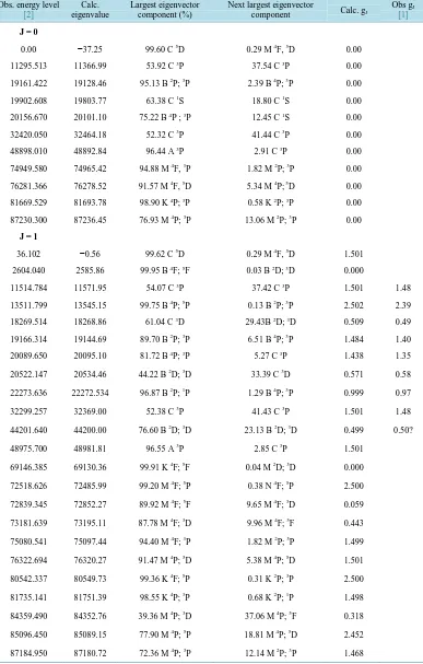
Table 1. Comparison between the observed and calculated energy levels (in∙cm−1) and gJ-factors. For each state the parent terms are given immediately after the configuration label in columns 3 & 4.

Obs. energy level

[2]

Calc. eigenvalue

Largest eigenvector component (%)

Next largest eigenvector

component Calc. gJ

Obs gJ

[1]

J = 0

0.00 −37.25 99.60 C 5D 0.29 M 4F, 5D 0.00

11295.513 11366.99 53.92 C 3_{P 37.54 C} 3_{P 0.00}

19161.422 19128.46 95.13 B 2_P; 3_{P 2.39 B} 4_P; 3_{P 0.00}

19902.608 19803.77 63.38 C 1_{S 18.80 C} 1_{S 0.00}

20156.670 20101.10 75.22 B 4_{P ;} 3_{P 12.45 C} 1_{S 0.00}

32420.050 32464.18 52.32 C 3P 41.44 C 3P 0.00

48898.010 48892.84 96.44 A 3_{P 2.91 C} 3_{P 0.00}

74949.580 74965.42 94.88 M 4_F, 3_{P 1.82 M} 2_P; 3_{P 0.00}

76281.366 76278.52 91.57 M 4_F, 5_{D 5.34 M} 4_P; 5_{D 0.00}

81669.529 81693.78 98.90 K 4_P; 3_{P 0.58 K} 2_P; 3_{P 0.00}

87230.300 87236.45 76.93 M 4P; 3P 13.06 M 2P; 3P 0.00

J = 1

36.102 −0.56 99.62 C 5_{D 0.29 M} 4_F, 5_{D 1.501}

2604.040 2585.86 99.95 B 4_F; 5_{F 0.03 B} 2_D; 3_{D 0.000}

11514.784 11571.95 54.07 C 3_{P 37.42 C} 3_{P 1.501 1.48}

13511.799 13545.15 99.75 B 4P; 5P 0.13 B 2P; 3P 2.502 2.39

18269.514 18268.86 61.04 C 3_{D 29.43B} 2_D; 3_{D 0.509 0.49}

19166.314 19144.69 89.70 B 2_P; 3_{P 6.51 B} 4_P; 3_{P 1.484 1.40}

20089.650 20095.10 81.72 B 4_P; 3_{P 5.27 C} 3_{P 1.438 1.35}

20522.147 20534.46 44.22 B 2_D; 3_{D 33.39 C} 3_{D 0.571 0.58}

22273.636 22272.534 96.87 B 2P; 1P 1.29 B 4P; 3P 0.999 0.97

32299.257 32369.00 52.38 C 3_{P 41.43 C} 3_{P 1.501 1.48}

44201.640 44200.00 76.60 B 2_D; 3_{D 23.13 B} 2_D; 3_{D 0.499 0.50?}

48975.700 48981.81 96.55 A 3_{P 2.85 C} 3_{P 1.501}

69146.385 69130.36 99.91 K 4_F; 5_{F 0.04 M} 2_D; 3_{D 0.000}

72518.626 72485.99 99.20 M 4_F; 5_{P 0.38 N} 4_F; 5_{P 2.500}

72839.345 72852.27 89.92 M 4F; 5F 9.65 M 4F; 3D 0.059

73181.639 73195.11 87.78 M 4_F; 3_{D 9.96 M} 4_F; 5_{F 0.443}

75080.541 75097.44 94.40 M 4_F; 3_{P 1.82 M} 2_P; 3_{P 1.499}

76322.694 76320.27 91.47 M 4_P; 5_{D 5.38 M} 4_P; 5_{D 1.501}

80542.337 80549.73 99.36 K 4_F; 5_{P 0.31 K} 2_P; 3_{P 2.500}

81735.141 81751.39 98.55 K 4_P; 3_{P 0.68 K} 2_P; 1_{P 1.498}

84359.490 84352.76 39.36 M 4P; 3D 37.06 M 4P; 5F 0.318

85096.450 85089.15 77.90 M 4_P; 5_{P 18.81 M} 4_P; 5_{D 2.452}

Continued

J = 2

106.643 70.89 99.64 C 5_{D 0.29 M} 4_F; 5_{D 1.501}

2687.208 2665.31 99.95 B 4_F; 5_{F 0.02 B} 2_D; 3_{D 1.000 0.97}

8640.362 8668.69 94.36 B 4_F; 3_{F 4.45 C} 3_{F 0.666 0.65}

11908.261 11977.54 54.12 C 3_{P 37.09 C} 3_{P 1.501 1.49}

13490.883 13467.88 69.00 C 3_{F 23.80 C} 3_{F 0.666 0.59}

13594.723 13623.51 99.58 B 4_P; 5_{P 0.22 B} 2_P; 3_{P 1.834 1.78}

18293.871 18294.96 63.00 C 3_{D 27.31 B} 2_D; 3_{D 1.172 1.13}

19132.791 19122.80 80.94 B 2_P; 3_{P 13.70 B} 4_P; 3_{P 1.486 1.38}

20343.046 20335.14 68.38 B 4_P; 3_{P 9.95 B} 2_D; 3_{D 1.439 1.36}

20617.073 20627.27 36.11 B 2_D; 3_{D 20.10 C} 3_{D 1.213 1.25}

20980.927 20993.21 37.78 B 2_D; 1_{D 32.50 C} 1_{D 1.027 1.02}

25191.035 25150.22 36.51 C 1_{D 33.78 B} 2_D; 1_{D 1.000 0.99}

30267.511 30257.99 38.55 C 3_{F 22.71 B} 2_F; 3_{F 0.666 0.67}

30673.088 30669.40 76.09 B 2_F; 3_{F 15.57 C} 3_{F 0.666 0.67}

32040.635 32115.49 52.52 C 3_{P 41.26 C} 3_{P 1.501 1.38}

37937.694 37933.75 76.22 A 3_{F 18.91 C} 3_{F 0.666}

44657.941* _{44105.45 60.81 A} 1_{D 22.76 C} 1_{D 1.001}

44159.460 44185.34 76.77 B 2_D; 3_{D 22.67 B} 2_D; 3_{D 1.167 1.14}

47324.288 47302.16 70.03 B 2_D; 1_{D 22.38 B} 2_D; 1_{D 1.001}

49204.650 49190.71 95.74 A 3_{P 2.60 C} 3_{P 1.496}

50951.660 50930.31 48.61 C 1_{D 32.62 C} 1_{D 1.003}

69228.318 69214.03 99.55 K 4_F; 5_{F 0.38 K} 4_F; 3_{F 0.999}

70415.542 70397.31 99.16 K 4_F; 3_{F 0.38 K} 4_F; 5_{F 0.667}

72674.924 72643.66 98.63 M 4_F; 5_{P 0.49 M} 4_F; 3_{D 1.831}

72878.056 72868.91 59.43 M 4_F; 5_{G 36.08 M} 4_F; 5_{F 0.604}

73027.311 73026.02 55.47 M 4_F; 5_{F 38.44 M} 4_F; 5_{G 0.738}

73310.069 73294.71 90.74 M 4_F; 3_{D 4.04 M} 4_F; 5_{F 1.162}

75335.879 75355.16 94.09 M 4_F; 3_{P 1.72 M} 2_P; 3_{P 1.500}

75813.489 75805.22 92.33 M 4_F; 3_{F 2.96 M} 2_G; 3_{F 0.668}

76403.674 76403.25 91.33 M 4_F; 5_{D 4.73 M} 4_P; 5_{D 1.501}

80623.249 80633.56 98.95 K 4_P; 5_{P 0.60 K} 2_P; 3_{P 1.833}

81914.328 81918.43 99.16 K 4_P; 3_{P 0.21 L} 4_P; 3_{P 1.501}

84406.210 84451.41 43.57 M 4_P; 3 _{D 26.93 M} 2_G; 3_{D 1.126}

85045.572 85043.16 83.87 M 4_P; 5_{P 13.43 M} 4_P; 5_{D 1.812}

86001.530 86003.05 29.26 M 4_P; 3_{F 26.59 M} 2_G; 3_{F 0.787}

Continued

J = 3

208.790 176.03 99.65 C 5_{D 0.29 M} 4_F; 5_{D 1.501}

2808.959 2784.06 99.95 B 4_F; 5_{F 0.02 B} 4_F; 3_{F 1.251 1.20}

8842.050 8860.61 94.04 B 4_F; 3_{F 4.72 C} 3_{F 1.083 1.04}

13542.645 13515.81 67.97 C 3_{F 23.09 C} 3_{F 1.079 1.06}

13741.640 13753.15 99.89 B 4_F; 5_{P 0.03 M} 4_F; 5_{P 1.668 1.62}

14461.748 14501.41 60.98 C 3_{G 36.44 B} 2_G; 3_{G 0.754 0.74}

16340.981 16372.76 62.73 B 2_G; 3_{G 36.14 C} 3_{G 0.750 0.76}

18353.827 18330.97 68.46 C 3_{D 24.53 B} 2_D; 3_{D 1.334 1.30}

20622.983 20668.95 52.95 B 2_D; 3_{D 30.24 C} 3_{D 1.334 1.26}

26839.749 26638.09 90.37 C 1_{F 8.13 B} 2_F; 1_{F 1.000 0.97}

30306.389 30299.56 33.57 C 3_{F 32.42 B} 2_F; 3_{F 1.083 1.06}

30641.767 30647.98 65.93 B 2_F; 3_{F 21.59 C} 3_{F 1.083 1.05}

34228.852 34216.02 91.47 B 2_F; 1_{F 8.11 C} 1_{F 1.000 1.00}

38193.021 38185.64 77.69 A 3_{F 17.89 C} 3_{F 1.084}

44098.473 44121.78 77.37 B 2_D; 3_{D 22.33 B} 2_D; 3_{D 1.334}

69352.530 69341.00 99.36 K 4_F; 5_{F 0.59 K} 4_F; 3_{F 1.250}

70629.831 70616.64 98.96 K 4_F; 3_{F 0.59 K} 4_F; 5_{F 1.084 1.06}

72448.600 72439.34 98.32 M 4_F; 5_{H 0.75 M} 4_F; 5_{G 0.503}

72908.997 72881.92 97.83 M 4_F; 5_{P 1.39 M} 4_F; 3_{D 1.663}

72951.558 72937.71 77.16 M 4_F; 5_{G 44.68 M} 4_F; 5_{F 1.118}

73146.343 73128.86 76.27 M 4_F; 5_{F 45.04 M} 4_F; 5_{G 1.046}

73530.712 73517.55 94.14 M 4_F; 3_{D 1.82 M} 4_P; 3_{D 1.337}

75422.910 75412.58 92.32 M 4_F; 3_{G 2.20 M} 2_G; 3_{G 0.757}

75966.119 75963.84 90.07 M 4_F;3_{F 3.05 M} 2_G; 3_{F 1.077}

76521.357 76522.23 91.27 M 4F; 5D 4.84 M 4P; 5D 1.501

80782.426 80783.98 99.62 K 4_F; 5_{P 0.23 M} 4_P; 5_{P 1.668}

81263.626 81321.39 99.91 K 2_G; 3_{G 0.02 L} 2_G; 3_{G 0.750}

84459.916 84504.10 53.04 M 4P; 3D 27.87 M 2G; 3D 1.307

84643.381 84670.91 86.67 M 2_G; 1_{F 7.33 M} 2_G; 3_{G 0.983}

84999.355 85012.56 89.91 M 4_P; 5_{P 6.53 M} 4_P; 5_{D 1.655}

85076.720 85088.67 82.85 M 2G; 3G 8.16 M 2G; 1F 0.772

86113.793 86098.83 46.73 M 2_G; 3_{F 35.01 M} 4_P;3_{F 1.096}

90381.370 90328.91 54.69 M 2_H; 1_{F 26.04 M} 2_D; 1_{F 0.998}

Continued

J = 4

339.125 310.43 99.63 C 5D 0.29 M 4F; 5D 1.501

2968.389 2941.09 99.96 B 4_F; 5_{F 0.02 B} 4_F; 3_{F 1.351 1.30?}

9097.889 9106.94 93.55 B 4_F; 3_{F 5.12 C} 3_{F 1.250 1.22}

12545.100 12622.67 97.95 C 3_{H 0.68 B} 2_H; 3_{H 0.801 0.83?}

13608.939 13583.18 67.66 C 3_{F 22.40 C} 3_{F 1.246 1.19}

14556.068 14595.48 60.41 C 3_{G 36.44 B} 2_G; 3_{G 1.052 1.00}

16421.528 16456.92 62.28 B 2_G; 3_{G 35.98 C} 3_{G 1.050 1.03}

17910.913 17867.69 50.71 C 1_{G 24.10 C} 1_{G 1.000 0.95}

19112.929 19115.38 73.06 B 2_G; 1_{G 11.99 C} 1_{G 0.995 0.98}

20242.382 20227.53 96.35 B 2_H; 3_{H 2.52 B} 2_G; 1_{G 0.806 0.82}

30318.528 30322.35 35.04 C 3_{F 32.06 B} 2_F; 3_{F 1.251 1.25}

30613.910 30628.55 52.07 B 2_F; 3_{F 30.39 C} 3_{F 1.251 1.23}

36424.870 36385.28 58.77 C 1_{G 35.58 C} 1_{G 1.000 0.96}

38517.080 38512.88 79.22 A 3_{F 16.63 C} 3_{F 1.250}

53607.200 53615.63 96.56 A 1_{G 2.86 C} 1_{G 1.000}

69518.528 69513.26 99.47 K 4_F; 5_{F 0.47 K} 4_F; 3_{F 1.350}

70898.570 70896.31 99.04 K 4_F; 3_{F 0.47 K} 4_F; 5_{F 1.251 1.23}

72551.297 72541.81 97.53 M 4_F; 5_{H 1.39 M} 4_F; 5_{G 0.904}

73063.719 73048.13 50.08 M 4_F; 5_{G 49.00 M} 4_F; 5_{F 1.249}

73279.343 73269.52 51.31 M 4F; 5F 48.49 M 4F; 5G 1.249

75140.638 75161.09 93.03 M 4_F; 3_{H 1.98 M} 4_F; 3_{G 0.805}

75615.397 75611.13 89.92 M 4_F; 3_{G 2.54 M} 4_F; 3_{F 1.051}

76143.052 76148.98 89.63 M 4F; 3F 3.25 M 2G; 3F 1.245

76673.101 76776.57 91.15 M 4_F; 5_{D 4.96 M} 4_P; 5_{D 1.501}

81343.015 81401.08 97.12 K 2_G; 3_{G 2.73 K} 2_{G ;} 1_{G 1.049}

82025.721 82075.24 96.61 K 2_G; 1_{G 2.76 K} 2_G; 3_{G 1.001}

85060.717 85083.03 85.44 M 2G; 3G 3.43 M 2H; 3G 1.041

85159.641 85168.02 90.41 M 2_G; 3_{H 5.61 M} 2_H; 3_{H 0.805}

86028.099 85974.94 99.40 K 2_H; 3_{H 0.29 K} 2_G; 1_{G 0.801}

86211.050 86215.96 49.90 M 2_G; 3_{F 34.78 M} 4_P; 3_{F 1.249}

87457.980 87494.83 69.77 M 2G; 1G 19.46 M 2D; 1G 1.003

Continued

J = 5

3162.966 3129.47 99.95 B 4_F; 5_{F 0.04 B} 2_G; 3_{G 1.401 1.28?}

12621.485 12702.6 98.13 C 3_{H 0.68 B} 2_H; 3_{H 1.034 1.02}

14655.607 14690.69 62.29 C 3_{G 36.07 B} 2_G; 3_{G 1.200 1.17}

16532.983 16569.48 62.99 B 2_G; 3_{G 35.75 C} 3_{G 1.200 1.16}

20280.251 20274.02 98.99 B 2_H; 3_{H 0.68 C} 3_{H 1.034 1.01}

23391.150 23410.26 99.71 B 2H; 1H 0.12 K 2H; 1H 1.000 1.04

69724.236 69729.28 99.91 K 4_F; 5_{F 0.05 K} 2_G; 3_{G 1.401 1.39}

72680.856 72672.75 97.24 M 4_F; 5_{H 1.65 M} 4_F; 5_{G 1.104}

73223.351 73206.48 53.20 M 4F; 5G 44.80 M 4F; 5F 1.326

73417.330 73417.60 53.98 M 4_F; 5_{F 44.70 M} 4_F; 5_{G 1.339}

75346.306 75383.89 93.06 M 4_F; 3_{H 1.92 M} 4_F; 3_{G 1.037}

75854.219 75861.13 92.60 M 4_F; 3_{G 2.03 M} 2_G; 3_{G 1.197}

81483.278 81541.61 99.50 K 2_G; 3_{G 0.22 K} 2_H; 3_{H 1.200}

84742.170 84771.02 97.89 M 2_G; 3_{I 1.43 M} 2_H; 3_{I 0.833}

84896.899 84927.93 90.38 M 2_G; 1_{H 6.46 M} 2_G; 3_{G 1.004}

85140.362 85162.11 84.54 M 2G; 3G 3.85 M 2H; 3G 1.192

85301.938 85308.03 82.79 M 2_G; 3_{H 7.49 M} 2_G; 1_{H 1.035}

86091.728 86039.72 97.94 K 2_H; 3_{H 1.74 K} 2_H; 1_{H 1.033}

86766.880 86695.84 96.71 K 2H; 1H 1.82 K 2H; 3H 1.001

88939.995 88915.30 97.24 M 2_H; 3_{I 1.52 M} 2_G; 3_{I 0.834}

89053.341 89027.95 92.39 M 2_H; 1_{H 2.50 M} 2_D; 3_{G 1.008}

J = 6

12706.078 12789.28 99.04 C 3_{H 0.69 B} 2_H; 3_{H 1.167 1.27?}

19191.326 19194.69 99.15 C 1_{I 0.45 M} 2_H; 1_{I 1.000 0.96?}

20363.335 20362.12 99.21 B 2H; 3H 0.69 C 3H 1.167 1.14

72837.581 72833.32 97.72 M 4_F; 5_{H 1.25 M} 4_F; 5_{G 1.216}

73499.773 73440.60 98.00 M 4_F; 5_{G 1.26 M} 4_F; 5_{H 1.332}

75592.481 75643.20 94.82 M 4_F; 3_{H 1.89 M} 2_H; 3_{H 1.167}

84859.580 84883.73 97.83 M 2_G; 3_{I 1.23 M} 2_H; 3_{I 1.024}

85415.904 85440.02 91.53 M 2_G; 3_{H 5.15 M} 2_H; 3_{H 1.166}

86191.750 86143.63 99.86 K 2_H; 3_{H 0.05 M} 2_G; 3_{H 1.167}

86453.764 86471.68 87.34 M 2_G; 1_{I 10.63 M} 2_H; 1_{I 1.000}

89005.580 89013.81 97.89 M 2_H; 3_{I 1.26 M} 2_G; 3_{I 1.024}

94371.80 94306.91 80.48 M 2_H; 1_{I 8.89 M} 2_G; 1_{I 1.000}

J = 7

73021.143 73024.65 99.28 M 4_F; 5_{H 0.61 N} 4_F; 5_{H 1.286}

85004.880 85002.77 98.25 M 2_G; 3_{I 1.01 M} 2_H; 3_{I 1.143}

89082.769 89094.38 98.38 M 2_H; 3_{I 0.99 M} 2_G; 3_{I 1.143}

J = 8

90180.86 99.57 M 2_H; 3_{K 0.43 N} 2_H; 3_{K 1.125}

A: 3d2_4s2 _{configuration; B: 3d}3_{4s configuration; C: 3d}4 _{configuration; K: 3d}3_{5s configuration; L: 3d}3_{6s configuration; M: 3d}3_4d

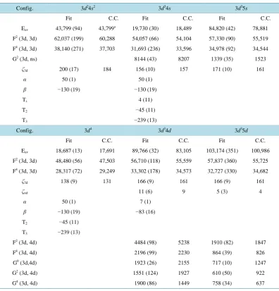
Table 2. Fine structure fitted parameters values (in∙cm−1) for the even-parity levels of V II (Fit) with their un-certainties in parentheses and for comparison their corresponding ab initio values computed by means of the Cowan code (C.C.). See also text.

Config. 3d2_4s2 _3d3_{4s 3d}3_5s

Fit C.C. Fit C.C. Fit C.C.

Eav 43,799 (94) 43,799a 19,730 (30) 18,489 84,820 (42) 78,881

F2 _{(3d, 3d) 62,037 (199) 60,288 54,057 (66) 54,104 57,330 (90) 55,519}

F4 _{(3d, 3d) 38,140 (271) 37,703 31,693 (236) 33,596 34,978 (92) 34,544}

G2 _{(3d, ns) 8144 (43) 8207 1339 (35) 1523}

ζ3d 200 (17) 184 156 (10) 157 171 (10) 161

α 50 (1) 50 (1)

β −130 (19) −130 (19)

Ts 4 (11)

T2 −45 (11)

T3 −239 (13)

Config. 3d4 _3d3_{4d 3d}3_5d

Fit C.C. Fit C.C. Fit C.C.

Eav 18,687 (13) 17,691 89,766 (32) 83,105 103,174 (351) 100,986

F2 _{(3d, 3d) 48,480 (56) 47,503 56,710 (118) 55,559 57,837 (360) 55,725}

F4 _{(3d, 3d) 28,317 (72) 29,249 33,302 (178) 34,573 32,727 (330) 34,682}

ζ3d 138 (9) 131 166 (9) 161 166 (9) 161

ζnd 11 (6) 9 5 (3) 4

α 50 (1) 7 (1)

β −130 (19) −83 (16)

T2 −45 (11)

T3 −239 (13)

F2 _{(3d, 4d) 4484 (98) 5238 1910 (82) 1847}

F4 _{(3d, 4d) 2196 (99) 2230 864 (39) 826}

G0 _{(3d,4d) 1923 (26) 2155 717 (10) 1247}

G2 _{(3d, 4d) 1551 (124) 1927 610 (50) 922}

G4 _{(3d, 4d) 1900 (86) 1449 758 (34) 637}

a

Fixed to the fitted value.

Table 3. Fine structure configuration interaction parameters and for comparison their corresponding ab initio

values computed by means of the Cowan code (C.C.).

Values of main configuration interaction parameters Fit C.C.

3d2_4s2 _{- 3d}3_{4s R}2 _{(3d3d, 3d4s)}

3d24s2 - 3d4 R2 (4s4s, 3d3d) 3d3_{4s - 3d}4 _R2 _{(3d4s, 3d3d)}

3d34d - 3d35d R2 (3d4d, 3d5d) R4 _{(3d4d, 3d5d)}

3d3_{4s - 3d}3_{4d R}2 _{(3d4s, 3d4d)}

3d4 _{- 3d}3_{4d R}2 _{(3d3d, 3d4d)}

R4 _{(3d3d, 3d4d)}

3d3_{5s - 3d}3_{4d R}2 _{(3d5s, 3d4d)}

3d2_4s2 _{- 3d}3_{4d R}2 _{(4s4s, 3d4d)}

−1960 (192) −4679

11869 (82) 11839

−4741 (42) −6813

2205 (173) 2606

1853 (253) 1288

4564 (320) 4109

6185 (380) 8434

3043 (583) 5580

−320 (70) −321

Table 4. Predicted singlet, triplet and quintet positions for missing experimental energy levels of the configu-rations mentioned in Table 2.

Configuration Designation J value Energy (cm−1) Composition LS (%)

3d4 1

S

0 60,212 65.7

3d2_4s2 1_S

0 77,196 89.6

3d34d (4_P) 5_F

1 84,407 63.7

2 84,376 65.8

3 84,427 76.7

4 84,503 98.0

5 84,599 98.6

(4_P) 5_D

0 85,178 91.8

1 85,221 89.1

2 85,260 88.2

3 85,291 89.3

4 85,313 91.2

(2_G) 3_D

1 86,241 52.5

2 86,359 30.1

3 86,346 36.9

(4P) 3F

2 86,536 A.G.E. 28.8

3 86,624 36.8

4 86,806 44.3

(2P) 3D

1 87,969 67.4

2 88,102 69.5

3 88,420 41.8

(2_D) 3_G

3 88,968 47.3

4 89,005 56.2

Continued

(2_P) 3_F

2 89,031 40.4

3 89,204 35.8

4 89,386 42.1

(2_D) 3_F

2 89,966 32.8

3 89,988 31.9

4 90,015 35.8

(2_H) 3_K

6 89,998 99.2

7 90,072 97.2

8 90,180 99.6

(2_H) 3_G

3 90,608 70.3

4 90,726 68.8

5 90,813 71.5

(2_D) 3_P

0 90,707 59.6

1 90,840 56.7

2 91,075 48.3

(2_D) 3_D

1 91,494 42.8

2 91,440 35.9

3 91,354 44.5

(2_H) 3_H

4 91,203 85.1

5 91,278 86.1

6 91,351 87.2

(2_D) 1_S

0 94,473 71.6

(2P) 1P

1 87,655 51.5

(2_D) 1_P

1 89,006 49.4

(2_D) 1_D

2 90,040 67.8

Continued

2 92,624 59.6

(2_P) 1_F

3 88,207 36.4

(2_D) 1_G

4 93,122 31.1

(2_H) 1_K

7 90,605 97.8

3d3_5s

(2P) 3P

0 84,728 98.8

1 84,741 94.9

2 84,793 88.1

(2_D) 3_D

1 85,873 49.8

2 85,809 68.5

3 85,888 76.6

(2_F) 3_F

2 96,784 99.8

3 96,740 99.0

4 96,690 99.8

(2_P) 1_P

1 85,233 68.0

(2F) 1F

3 97,299 98.8

A.G.E.: already given experimentally.

A good fit, with a root mean square uncertainty of 6.2 MHz was obtained. The values of the model space hfs

parameters, quoted with their uncertainties, are presented in

Table 5

. In order to check the validity of these fitted

parameters we have compared some of them to those computed using values obtained by means of the Cowan

code. For example one can use the well-established relation

a

(

MHz

)

2

r

4π

I

95.4128

g

r

κ κ

κ

₌

_{µ µ µ}

₌

.

Using the values of line 2 of

Table 6

, knowing that the nuclear spin and magnetic dipole moment of

V are

equal respectively to 7/2 and 5.1485

μ

one gets the

a

values of line 3 of

Table 6

which are on the whole

close to the experimental ones, located in line 1 of the same Table. This confirms the well-founded basis of our

work.

To check the value of the most influential hfs-deduced parameter,

a

(

3

d

4

s

)

, it is interesting to compare the

ratio

(

)

(

)

10 4 4 10 3 4

3

4

₂₅₃₅

0.56

4519.76

3

4

s

s

a

d

s

a

d

s

=

=

relative to V I

[13]

and V II (this work) with

(

)

(

)

3

4

₄₈₇

0.58

836.27

3

4

s

s

a

d

s

a

d

s

−

=

=

−

relative to Ti I

[14]

and Ti II

[7]

. Since these ratios are very close for these two neighbour elements in the Peri-

odic Table, we can conclude that the deduced

a

(

3

d

4

s

)

value for V II is really satisfactory. To extract

mag-netic dipole A-values from experimental hfs splitting the electric quadrupole hfs B factors preferably were fixed

deliberately to zero in

[12]

because the electric quadrupole moment of

V is small:

−0.05b. In this case it is not

useful to compute

nl

b

values since it is not possible to make comparisons between experimental and

theoreti-cal

nl

b

values.

Table 5. The fitted hfs many-body parameter values inMHz for the model space (3d + 4s)4. The uncertainties given in parentheses are the standard deviations.

01 3d

a 498.71 (6.62) a1 177.04 (6.45)

12 3d

a 469.24 (23.02) a2 51.34 (1.87)

10 3d

a −14.86 (9.33) a3 34.17 (1.24)

10 4s

a 4519.76 (130.78) a9 813.26 (36.93)

12

IC

a 44.50 (19.81) a11 −3617.15 (135.90)

a4 = a5 = a6 = a7 = a8 = a10 = 0.00 (fixed).

Table 6. Comparison between fitted and calculated hfs many-body parameter 01 3d

a in MHz. Radial integrals are computed by means of the pseudo-relativistic Cowan code.

Parameter 3d2_4s2 _3d3_{4s 3d}4

01 3d

a (Fit) (MHz) 427.90 357.09 286.27

<r−3>3d (a.u.) 3.018 2.615 2.233

01 3d

a (Cal) (MHz) 423.58 367.02 313.41

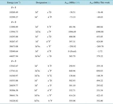
Table 7. Our computed hfs A-constants of V II (in MHz), compared with those obtained experimentally by Armstrong etal. [10].

Energy (cm−1) Designation [1] Aexp (MHz) [10] Acal (MHz) This work

J = 1

18269.49 3d4 _a 3_{D −38.51 −36.48}

32299.27 3d4 _d 3_{P −73.33 −69.03}

J = 2

13490.89 3d4

b 3F 481.96 480.84

13594.73 3d3_{4s a} 5_{P 1096.69 1098.88}

18293.88 3d4 _a 3_{D 488.08 453.85}

30267.47 3d4 _d 3_F* _{397.31 424.89}

30673.08 3d3_{4s c} 3_F* _{−250.92 −269.78}

32040.64 3d4 _d 3_{P 0 (fixed) −2.72}

44657.94 3d2

4s2 c 1D 365.79 379.22

J = 3

13542.67 3d4 _b 3_{F 250.91 255.18}

13741.61 3d3_{4s a} 5_{P 840.96 850.03}

16340.97 3d3_{4s b} 3_{G 138.66 148.39}

18353.88 3d4 _a 3_{D 502.93 494.22}

26839.77 3d4

a 1F 301.10 293.02

30306.38 3d4 _d 3_F* _{332.71 331.54}

30641.76 3d34s c 3F* 414.24 422.43

Continued

J = 4

13608.96 3d4 _b 3_{F 171.4 174.57}

16421.51 3d3_{4s b} 3_{G 423.32 416.55}

30318.55 3d4 _d 3_F* _{434.52 394.42}

30613.92 3d3_{4s c} 3_F* _{591.70 623.83}

38517.06 3d2_4s2 _e 3_{F 276.67 263.47}

J = 5

14655.63 3d4 _a 3_{G 436.10 452.52}

16533.00 3d3_{4s b} 3_{G 498.41 495.91}

*_{: See text.}

Table we inserted also our computed values which confirm totally the Armstrong, Rosner and Holt experimental

data

[12]

which are sometimes different from those of Arvidsson

[15]

. As regards the 3

d

4

s

e

F

(38517.06

cm

) hfs value we reject A=

−351.28 and we keep A= 276.67 MHz since two values were proposed in

[12]

(owing to an unavoidable ambiguity in ΔJ = 0 transitions).

3. Conclusion

Parametric fs studies including configuration interactions have been carried out for five interacting

configura-tions of V II. We furthermore propose predicted energy level values for missing experimental ones up to

100,000 cm

for further investigations. One can also note that calculated Landé g

-factors were also in good

agreement with the experimental ones. Unfortunately the latter are not as numerous as we might have expected

and thus our work to check level assignments became more difficult. We give for the first time the hfs many-

body parameter values with good accuracy for the model space (3

d +

4

s

)

, taking advantage of the accurate

work done in

[10]

. This provides better predictions for still unknown levels. The conclusive comparison between

the experimental and calculated hfs A-constants, given in

Table 7

, provides a good check on the quality of the

wave functions obtained by the least squares fit of the fine structure, used to determine the expansions of hfs

A-constants in intermediate coupling. Very recently the spectrum of V II has been recorded by FTS and thirty-

nine of the additional eighty-five high levels published by Iglesias

et al.

[3]

have been confirmed or revised, and

four of their missing levels have been found

[16]

as regards even-parity levels. One can note in our

Table 1

a

total agreement with the assignments of these four new levels given in this interesting work.

References

[1] Meggers, W.F. and Moore, C.E. (1940) Journal of Research of the National Bureau of Standards (US), 25, 83. [2] Sugar, J. and Corliss, C.H. (1985) Journal of Physical and Chemical Reference Data, 14, 1-664.

http://dx.doi.org/10.1063/1.555747

[3] Iglesias, L., Cabeza, M.I., Garcia-Riquelme, O. and Rico, F.R. (1987) Optica Pura y Aplicada, 2, 137.

[4] Bouazza, S. (2011) International Journal of Quantum Chemistry, 111, 3000-3007. http://dx.doi.org/10.1002/qua.22614 [5] Bouazza, S. (2012) International Journal of Quantum Chemistry, 112, 470-477. http://dx.doi.org/10.1002/qua.22974 [6] Bouazza, S. (2012) Physica Scripta, 86,015302. http://dx.doi.org/10.1088/0031-8949/86/01/015302

[7] Bouazza, S. (2013) Physica Scripta, 87,045301. http://dx.doi.org/10.1088/0031-8949/87/04/045301 [8] Bouazza, S. (2013) Physica Scripta, 87, 035302. http://dx.doi.org/10.1088/0031-8949/87/03/035302 [9] Cowan, R.D. (1981) The Theory of Atomic Structure and Spectra. University of California Press, Berkeley.

[10] Armstrong, N.M.R., Rosner, S.D. and Holt, R.A. (2011) Physica Scripta, 84, 055301. http://dx.doi.org/10.1088/0031-8949/84/05/055301

[11] Dembczynski, J. (1996) Physica Scripta, 65, 88.

4, 39.

[13] Palmeri, P., Biémont, E., Quinet, P., Dembczynski, J., Szawiola, G. and Kurucz, R.L. (1997) Physica Scripta, 55, 586. http://dx.doi.org/10.1088/0031-8949/55/5/011

[14] Aydin, R., Stachowska, E., Johann, U., Dembzynski, J., Unkel, P. and Ertmer, W. (1990) Zeitschrift für Physik D, 15, 281.

[15] Arvidsson, K. (2003) Master’s Thesis Lund Observatory. Lund University, Sweden.