Volume 74– No.1, July 2013
Designing Graph Database Models from Existing
Relational Databases
Subhrajyoti Bordoloi
Dept. Of Computer Applications Assam Engg. College, Guwahati, Assam
Bichitra Kalita
Dept. Of Computer Applications Assam Engg. College, Guwahati, Assam
ABSTRACT
In this paper, a method for transforming a relational database to a graph database model is described. In this approach, the dependency graphs for the entities in the system are transformed into star graphs. This star graph model is transformed into a hyper graph model for the relational database, which, in turn, can be used to develop the domain relationship model that can be converted in to a graph database model.
General Terms
Dependency Graph, Hypergraps, Graph Database, Reference Graph, Star Graph, Candidate keys,
Keywords
Tuple Dependencies (TuD), Domain Dependencies (DoD).
1.
INTRODUCTION
Graphs and hyper graphs are extensively used to describe various concepts in database technology- ranging from data modeling to data processing. There are many graph based approaches applied in RDBMS [1], 3], [13]. Recently the Graph Database is a hot topic of research in database technology [4], [6], [7], [9]. Graph database is becoming popular because it addresses a set of complex data related application domains such as WWW, social networking, genomics.[3][5][6][7][10][12] Hyper graphs and graphs are very much used in describing graph database structures, the complex interactions among the data[1][11]. The interactions among the data items forms a complex graph and the prime objective of graph database is to find a certain pattern(sub graph) in the complex graph using graph theory and graph algorithms. It is difficult to manage the complex interactions in relational databases and studies show that graph database is better than any RDBMS [3] [8].
In this paper, few concepts of graph oriented design methodologies used in DBMS are discussed. A novel method to construct graph database models from existing relational and object oriented database is proposed. For discussion, the SUPPLIER-PART database [2] is considered.
2.
GRAPH BASED APPROACH IN
DATABASE DESIGN
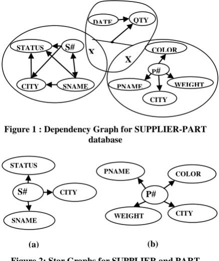
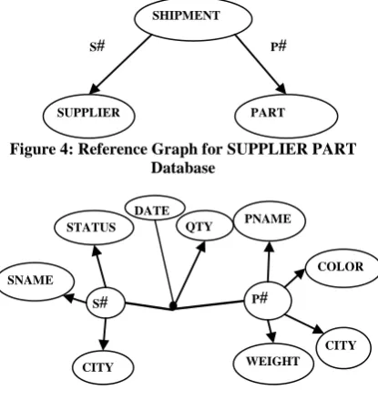
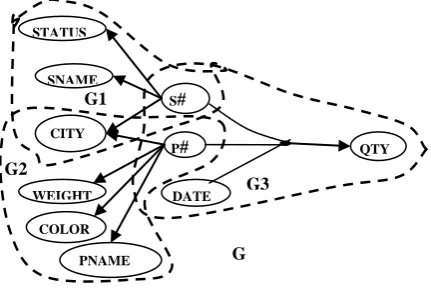
Figure 1 shows the dependency graph for the supplier-part database. Considering the dependencies available among the attributes of the entities, the candidate keys are identified [4]. For example, there are two candidate keys(S# and SNAME) for the entity SUPPLIER and one candidate key (P#) for the entity PART. Choosing S# as the primary key for SUPPLIER and P# for PART, the
star graphs for these entities as shown in Fig.2 are obtained.. This analysis will determine the attributes from the entities SUPPLIER and PART which will be included in the relationship set (intersecting portions marked as X in Fig.1.).
[image:1.595.314.533.249.510.2]Figure 1 : Dependency Graph for SUPPLIER-PART database
Figure 2: Star Graphs for SUPPLIER and PART
[image:1.595.336.512.596.655.2]Finally, a dependency graph for the relationship SHIPMENT as shown in Fig.3 (a) is obtained. From this dependency graph, the star graph for SHIPMENT can be drawn as shown in Fig.3 (b). Finally, the following reference graph for the database as shown in Fig.4 is obtained.
Figure 3: Dependency Graph and the Star Graph for SHIPMENT
QTY
S#,P#
DATE
S#, P#, DATE QTY
(a) (b)
SNAME
CITY
S#
CITY COLOR STATUS
WEIGHT PNAME
P#
(a) (b)
QTY
P#
CITY COLOR
PNAME WEIGHT DATE
X
X S#
SNAME STATUS
Figure 4: Reference Graph for SUPPLIER PART Database
Figure 5: Hyper Graph Model for SUPPLIER-PART Database
Figure 6: B-Arc Structure for SHIPMENT
3.
GRAPH DATA MODEL USING
TUPLE ORIENTED DEPENDENCY
The graph structure of the database can be deduced from the mathematical model [13] of the database. If xi be the
attributes in the key set, kSof the set S representing a
database table, then the central node of the star graph will contain xi. The mathematical model for the
SUPPLIER-PART database is as follows. DRS NAME = SUPPLIER-PART
SET SUPPLIER= {{{S#}},{{SNAME},{STATUS}, {CTIY}}}
SET PART = {{{P#}},{{PNAME},{COLOR}, {WEIGHT},{CITY}}}
SET SP = {{{S#},{P#},{DATE}},{{QTY}}}
To find the relationships among these sets (tables) take the intersection of the sets as follows.
SUPPLIER ∩ PART=φ --- (1) SHIPMENT ∩ SUPPLIER= {{S#}} --- (2a) {S#} Є KS --- (2b)
SHIPMENT ∩ PART= {{P#}} --- (3a) {P#} Є KP --- (3b)
[Note that, Equation 2(a) and Equation 3(a) can be obtained from the reference graph shown in Fig. 4]
From this it is found that there is a relationship (m: n) between SUPPLIER and PART through SHIPMENT. The central node of the star graph for SHIPMENT will contain S#, P#, DATE (see Fig.3 (b)). Therefore, a graph (hyper graph) representation of the database (see Fig.5) can be obtained from the mathematical model of the database. To convert the database to a graph (hyper graph) model, the mathematical model of the database is required. This mathematical model can also be obtained from the database tables in the system by using a reverse engineering approach [13] or from the schema diagram. Consider the following relational data model instance of the SUPPLIER-PART database.
Table 1: SUPPLIER
S# SNAME STATUS CITY
S1 RAM 20 KOLKOTTA
S2 HARI 20 KOLKOTTA
S3 BOB 40 MUMBAI
Table 2: PART
P# PNAME COLOR WEIGHT CITY
P1 NUT RED 12 KOLKOTTA
P2 BOLT GREEN 15 CHENNAI
P3 SCREW BLUE 13 MUMBAI
P4 BOLT RED 15 CHENNAI
Table 3: SHIPMENT
S# P# DATE QTY
S1 P1 1/1/13 100
S1 P2 1/1/13 200
S2 P1 1/1/13 200
S2 P3 2/1/13 300
S3 P1 2/1/13 300
S3 P3 2/1/13 200
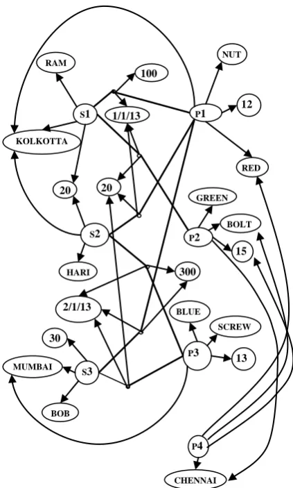
In Fig.7, nodes are created for each attribute values in the database instance. All nodes in this model are simple nodes. The hyper edges can also store information. The suppliers and the parts are connected by shipments, so the hyper edges can be labeled as shown in Fig.8. In this model, S1, S2, S3 are nodes representing star graphs for SUPPLIERs. P1, P2, P3, P4 that represent the nodes for PARTs. Moreover, the tuple oriented dependency is considered here. The attribute level dependencies are not considered
QTY S#
P#
DATE STATUS
SNAME S#
CITY
QTY DATE
CITY COLOR
WEIGHT PNAME
P#
SUPPLIER
P#
S#
Volume 74– No.1, July 2013
Figure 7: Hyper Graph Model for SUPPLIER-PART Database Instance using Tuple Oriented
[image:3.595.314.526.234.586.2]Dependencies.
Figure 8: The graph model for SUPPLIER-PART Database instance using Tuple Oriented
Dependencies
4.
GRAPH DATA MODELS USING
DOMAIN ORIENTED DEPENDENCY
Domain dependency is the dependency among the domain values. In this representation, number of nodes is substantially reduced, hence the complexity is reduced. A very small number of values from a domain are used several times in the database tables. The dependencies in the star graph and the relationships among the star graphs are also described by using the domain dependencies. So, a domain relationship diagram can be drawn to describe a relational database. The graph data model of Fig. 7 is represented using domain oriented dependencies as shown in Fig. 9.
Figure 9: Hyper Graph Model for SUPPLIER-PART database Instance using Domain Oriented
Dependencies.
The domain relationship model for the SUPPLIER-PART database is represented in Fig.10. The relationships among the domains of the attributes are considered. The prime focus is now the domains in the system, not the entities. Entities share domains. For example, as shown in Fig.10, entities SUPPLIER and PART share the same domain (CITY) values. Therefore, graph database model can be created from existing relational database by considering the relationships among domains in the system. The dependencies among the domains in the star graph can be 1: n or n: 1. For
P3
BLUE
13
S1
RAM
KOLKOTTA
S2
HARI
20
S3
BOB
30
MUMBAI
100
1/1/13
20 0
2/1/13
P2
GREEN
BOLT P1
RED NUT
12
P4 1
CHENNAI
300
15
SCREW
e5 2/1/13::300 e2 1/1/13::200
e3 1/1/13::200
e4 2/1/13::300 e1 1/1/13::100
e6 2/1/13::200
SUPPLIER SHIPMENT PART
S1*
S2
S3
P1
P3
P4
* Nodes include all information about a supplier P2
P3
MUMBAI BLUE
SCREW
13
S1
RAM
20
KOLKOTTA
S2
HARI
20
KOLKOTTA
S3
BOB
30
MUMBAI
1/1/13
100
1/1/13 20 0
1/1/1 3
200
2/1/13
2/1/13 300
2/1/13 200
P2
CHENNAI GREEN
BOLT
15
P1
KOLKOTTA
RED NUT
12
P4
CHENNAI
RED BOLT
[image:3.595.89.283.483.605.2]example, one CITY can be related to may S# or any number of P#.
Figure 10: Domain Relationship Model for SUPPLIER-PART Database
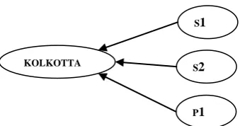
So, in the database instance for the SUPPLIER-PART database, only one node for one CITY value “KOLKOTTA” will be created and there may be many edges to connect it to many nodes for different S#-values and many different P# -values (See Fig. 11).
[image:4.595.79.284.96.204.2]
Figure 11: Connection of KOLKOTTA to three different S# vales and P# values
[image:4.595.93.263.344.433.2]For an m: n relationship, a hyper edge is created connecting the m-side key node, the n-side key node and the other key nodes to any dependent node. Note that, for the composite keys in the relational database, hyper edges are created to connect the nodes for the attributes (domains) in the composite keys to any node for dependent attributes (domains). Therefore, the domain relationship model can be represented as a hyper graph (see Fig. 12). If a graph model for a database instance of SUPPLIER-PART database is created, then this model will follow the structure as shown in Fig. 12.
Figure 12: Hyper graph model for Domain Relationship Diagram for SUPPLIER-PART
Database
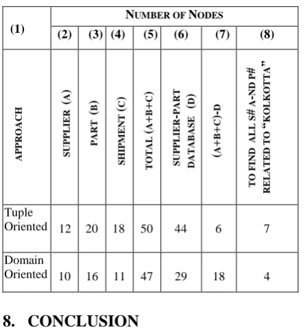
By considering the domain dependencies and creating only one node for a particular domain value appearing several times in a table (or in many tables), the data retrieval speed is enhanced and reduces the extra processing of node data as well. For example, consider the graph data model in Fig.8 and Fig.9. In the data model in Fig.8 a query to find all suppliers and parts in KOLKOTTA needs seven node accesses and lots of processing of node information. But in the data model in Fig.9, this query needs to locate the first supplier (links in the look-up index for S#) node which has a relationship to the node “KOLKOTTA” and once the node “KOLKOTTA” is located, all S#s and P#s can be located in constant time. This is because it is assumed that a node in the graph database knows which node(s) are at the other end of the edge (relationship). The dominating factor in the search is the time required to find the first node having the search-key or the node in the look-up index which has a relationship to the node having the search–key. In this case, the node for the search key “KOLKOTTA” is located through the first node in the look-up for S#. The number of node accessed is 4 in the model with domain oriented dependency, whereas, the number of node accessed is 7 in the model with tuple oriented dependency [see Table 4].
In the next section, a method to create a graph model for the database instance of a relational database is discussed.
5.
CREATING GRAPH MODEL FOR
A RELATIONAL DATABASE
INSTANCE
In this approach, the tables in the database are read once for a particular period (session) say for a day and a graph model is created for these data. This graph is stored in the server’s memory. All subsequent transactions are performed on this graph model. Adding data to the tables requires creating nodes for the domain values and creating edges to connect these nodes accordingly. If a node for the domain value is already in the graph we just need to create the appropriate edges in the graph to represent the relationship.
5.1
Creating the Domain Relationship
Diagram
If we observe the mathematical model, we cannot find the cardinality of the relationship directly. But the cardinality information is hidden in the model.
Let A and B are two set representing two tables in the database.
If A∩B=bi such that bi Є B and bi= kB but bi does not
belong to KA,where KA is the key set of A, then the
cardinality of the relationship between A and B is 1:1 or 1:n. Therefore the relationship between aj and bi is
assumed to be 1: n. Now, let us consider a set C (table) with kA and kB , where kA and kB are the keys of A and
B. If kA and kB does not belong to KC then there are two
relationships, one between A and C and the other between B and C which are 1: n, i.e. C is related with both A and B. If kA Є KC and kB Є KC , then there is one
m:n relationship between A and B. So, for independent set or the set having a 1: n relationship with other set, a 1: n relationship from each describing attribute to the key attribute in the set is created. For a derived set create an m: n relationship between the foreign keys of the sets. For all attributes in the key set of the derived set, create m: n relationship to the relationship created between the <PNAME>
<DATE>
<STATUS>
<QTY>
<SNAME>
<CITY> <WEIGHT>
<COLOR> <P#>
<S#>
COLOR S#
CITY SNAME
STATUS
P#
QTY DATE
WEIGHT PNAME
KOLKOTTA
S1
S2
[image:4.595.72.285.562.690.2]Volume 74– No.1, July 2013
MUMBAI
S1
RAM
20
KOLKOTTA
Figure 13: (b) A shipment of Part P3 by Supplier S3 Figure 13: (a) Graph models for Supplier S1
13
P3
MUMBAI BLUE
SCREW
S3
BOB
30 2/1/13
200
CITY CITY
WEIGHT COLOR DATE
SNAME
STATUS PNAME
QTY STATUS
SNAME CITY
foreign keys. For other attributes in the describing set of the derived set, create n: 1 relationship from the relationship created between the foreign keys.
5.2
Algorithm 1:
[Creating Domain Relationship model]
Step 1: Develop an E-R model by using reverse engineering approach. [13] Identify the unique domains for the attributes.
Step 2: Develop the Domain Relationship Model
2.1. For the entities create relationships (1: n) from
the key attribute to all describing attributes. For entities having composite key we get an n-ary relationship.
2.2 For n:1 relationship in the E-R model, create an 1:n relationship from the key of n-side entity to the key of the 1-side entity. For m:n relationship in the E-R model, create m:n n-ary relationship from the keys of the participating entities in the m:n relationship and other distinguishing attributes in the m:n relationship to the describing attributes of the m:n relationship.
5.3
Algorithm2:
[Creating Graph Database Model from
the Table data]
Step2: Read the table data and find the distinct domain values in the database.
Step3: Create nodes for these distinct domain values.
Step4: Create edges for the relationship following the Domain Relationship Diagram.
[image:5.595.82.445.53.703.2]For each row in a table create edges from the domain value for the key in the table to other non-key domain values and label the edge with the attribute names as shown in Fig. 13(a). If the table has composite key then create a hyper edge to connect the key domain values to other non-key domain values as shown in Fig. 13(b). [Fig.18 shows the complete graph data model created by following the Algorithm 2.]
6.
QUERYING DATA FROM THE
GRAPH MODEL
The graph data model for the SUPPLIER-PART database basically consists of four graph patterns G1, G2, G3 and G as shown in Fig.15. Querying from the database is now equivalent to mining sub graphs from the graph model.
Figure 14: Four Sub Graphs in SUPPLIER-PART Graph Database
6.1
Get all supplier details.
This query is equivalent to matching the graph pattern (G1) of Fig.15 from the graph data model.
Figure 15: Sub GraphG1 of the graph in Fig.14
QTY S#
P#
DATE CITY
COLOR
PNAME WEIGHT STATUS
SNAME
G3 G1
G2
G
S#
CITY STATUS
SNAME
[image:5.595.317.533.358.508.2] [image:5.595.346.497.598.697.2]QTY S#
P#
DATE
G3
6.2
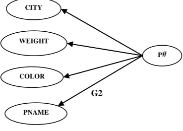
Get all parts details.
[image:6.595.92.527.82.425.2]This query is equivalent to matching the graph pattern (G2) of Fig.16 from the graph data model.
Figure 16: Sub Graph G2 of the graph in Fig.14
6.3
Get all shipments details.
This query is equivalent to matching the graph pattern (G3), shown in Fig.17, from the graph data model
[image:6.595.344.514.534.625.2]7.
COMPARISON OF THE
APPROACHES
Figure 17: Sub Graph G3 of the graph in Fig.14
A comparison between Tuple Oriented Dependency model and Domain Oriented Dependency model is shown in Table 4. The last column(8) of the table shows the number of nodes accessed to find all suppliers in KOLKOTTA and all parts produced in KOLKOTTA in the respective models. The number of nodes required to model the data in table SUPPLIER in tuple oriented model is 12 and 10 in the domain oriented model. If the complete database is modeled in tuple oriented approach the number of nodes is 44 whereas the number of nodes is 29 in domain oriented approach for the complete database (see column 6 in Table 4).
P#
CITY
COLOR
PNAME WEIGHT
G2
BLUE
SCREW
13
S1
RAM
KOLKOTTA
S2
HARI
20
BOB
30
MUMBAI
1/1/13
100
200
300
P2
CHENNAI GREEN
BOLT P1
RED
NUT
12
P4 2/1/13
15
SNAME SNAME
SNAME
PNAME
PNAME PNAME
PNAME STATUS
STATUS
STATUS
CITY
COLOR
CITY CITY
CITY
CITY
COLOR COLOR
WEIGHT WEIGHT
WEIGHT COLOR
CITY
WEIGHT DATE
DATE
DATE
DATE DATE QTY
QTY
QTY
QTY S#
S#
S#
S#
S#
S#
P#
P#
P#
P#
QTY QTY
P#
S3 P3
[image:6.595.95.280.550.682.2]DATE
Figure 18: Hyper Graph Model for SUPPLIER-PART Database Instance Using Domain Dependencies
Volume 74– No.1, July 2013
Table 4: Nodes Requirements for individual Tables and the Database
8.
CONCLUSION
In this paper, an approach to design graph database model from existing relational databases is discussed. This approach can be used to design new graph databases models. This approach can also be applied to derive graph database models from existing object-oriented databases. This approach can also be automated. Study is going on to implement it by using Neo4j graph database.
9.
REFERENCES
[1] Ronald Fagin , “Degrees of Acyclicity for Hypergraphs and Relational Database Schemes”, Journal of the Association for Computing Machinery,Vol-30, No 3, July 1983, pp 514-550 . [2] C.J.Date, “An Introduction to Database System” 3rd
Edition,Vol. 1, Addison-Wesley/Narosa Indian Student Edition, ISBN 85015-58-9 .
[3] J. Fong, H.K. Wong, Z. Cheng ,”Converting relational database into XML documents with DOM” Information and Software Technology 45(2003)335 –355.
[4] S.G. Shrinivas et. al. “APPLICATIONS OF GRAPH THEORY IN COMPUTER SCIENCE AN OVERVIEW” International Journal of Engineering Science and Technology Vol. (9), 2010, 4610-4621. [5] Philippe Cudré-Mauroux,Sameh Elniketyt. ”Graph
Data Management Systems for New Application Domains” Proceedings of the VLDB Endowment, Vol. 4, No. 12, 2011.
[6] Darshana Shimpi ,Sangita Chaudhari “An overview of Graph Databases”, International Conference in Recent Trends in Information Technology and Computer Science (ICRTITCS - 2012) Proceedings published in International Journal of Computer Applications® (IJCA) (0975 – 8887.
[7] Michal Laclavík ,et. al.,“Emails as Graph: Relation Discovery in Email Archive”WWW2012 Companion, April 16–20, 2012, Lyon, France. ACM 978-1-4503-1230-1/12/04.
[8] Shalini Batra, Charu Tyagi ,“Comparative Analysis of Relational And Graph Databases” International Journal of Soft Computing and Engineering (IJSCE) Volume-2, Issue-2, May 2012 ,pp-509-512. [9] Sherry Verma “ COMPARING MANUAL AND
AUTOMATIC NORMALIZATION
TECHNIQUES FOR RELATIONAL DATABASE ”International Journal of Research in Engineering & Applied Sciences,Vol- 2,Issue -2 , 2012, pp 59-67. [10] Prashish Rajbhandari, et. al.,“Graph Database
Model for Querying, Searching and Updating“, International Conference on Software and Computer Applications (ICSCA) ,2012 ) ,vol-41,pp-170-175. [11] Mike Buerli,“The Current State of Graph
Databases” Department of Computer Science, Cal Poly San Luis Obispo,[email protected], December 2012.
[12] Borislav Iordanov, HyperGraphDB: A eneralized GraphDatabase”Kobrixsoftware,Inc.http://www.kob -rix.com, Lecture Notes in Computer Science: HyperGraphDB .
[13] S. Bordoloi, B. Kalita, “E-R Model to an Abstract Mathematical Model for Database Schema using Reference Graph”, International Journal of Engineering Research and Development, 2013, Vol 6, Issue 4, pp. 51-60.
(1)
NUMBER OF NODES
(2) (3) (4) (5) (6) (7) (8)
AP P ROAC H S UP P L IE R ( A ) P AR T ( B ) S HI P M E NT ( C ) T OT AL ( A + B + C ) S UP P L IE R -P AR T DA T AB ASE ( D ) ( A + B + C )-D T O F IND AL L S # A -ND P # RE L AT E D T O “ KO L KO T T A ” Tuple
Oriented 12 20 18 50 44 6 7
Domain