Estimation of Ready Queue Processing Time using Transformed Factor Type (T F T) Estimator in Multiprocessor Environment

(1)

Estimation of Ready Queue Processing Time using

Transformed Factor-Type (T-F-T) Estimator in

Multiprocessor Environment

Diwakar Shukla

Deptt. of Mathematics and Statistics, H.S. Gour Central University, Sagar, M.P, India

Anjali Jain

Deptt. of Computer Sc. and Applications

H.S. Gour Central University Sagar, M.P, India

Kapil Verma

Deptt. of Computer Science M. P. Bhoj (Open) University

Bhopal, M.P, India

ABSTRACT

The ready queue processing time estimation problem appears when many processes remain in the ready queue just before the occurrence of sudden failure of system. The system administrator has to decide immediately, how much further time is required to process the remaining jobs in the ready queue, before shutting down the entire system as precautionary measure, so that while restart, it may remain in the safe state. In lottery scheduling, this prediction is possible with the help of sampling techniques. Factor- Type estimation method, existing in literature of sampling, was used by many authors to predict the time required provided the highly correlated sources of auxiliary information are available. This paper suggests two new estimation methods to predict the remaining total processing time required to process completely the ready queue provided sources of auxiliary information are negatively correlated. Under this approximation, the bias and m.s.e of the proposed estimators have been obtained using the set up of random sampling applicable to lottery scheduling. Performance of both estimation methods are compared in terms of mean squared error. The confidence intervals are calculated for comparing the efficiency of the estimate. One proposed estimator found better over other. .

Keywords

Lottery Scheduling, Transformed Factor-Type (T-F-T) Estimator, Mean Squared Error (M.S.E), Variance, Confidence Intervals

1. INTRODUCTION

Suppose there are k processors in a multiprocessor and multi-user environment and a large number of processes, say N, are in waiting queue. The CPU scheduler adopts lottery scheduling procedure to choose randomly any n processes from the waiting queue



_n



_N



and allocates to k processors



_n



_k



in sequential manner. The Lottery scheduling is different from basic scheduling algorithm, where each process is allocated a number of lottery tickets determining the possibility of process when to use the CPU. At each schedule point, a lottery is held and the process in the ready queue with the winning ticket gets the CPU utilization. Unlike priority scheduling, every job has equal chance of being represented to the processors [1] [2]. A technical problem appears when N is very large and because of the congestion, many processes have to wait until they called in random manner. If all of sudden the system collapses due to failure of power supply, maintenance problem, technical faults or due to any other unavoidable

much additional time require for finishing the remaining processes so that after restart the system remains in safe state. Such predictions are uncertain and require probability mechanism to resolve. Processor queues are matrices and Microsoft Windows (NT, 2000, XP) maintains its registry. To predict system behavior and CPU queue length, Microsoft NT, Windows 2000 developed a queuing theory model and derived fair share scheduling which guarantees application performance by explicitly allocating share of system resources among competing workloads [3]. Observed values (auxiliary information) often contradict expectations about how queue length should correlate to the system load (e.g. CPU utilization or burst time, transaction response time, process priority etc.) [4,5]. In literature it is common and well known idea that often more input information provides better prediction subject to condition when information are related whether positively or negatively [6, 7]. In order to obtain ready queue length time estimate, the authors in [8] proposed usual lottery scheduling (ULS) procedures in multiprocessor environment where variable of main interest (i.e. processing time) and auxiliary information like size of the process was positively correlated.

In [9], the authors describes systematic lottery SL-Scheduling scheme, to improve upon the prediction of ready queue processing time.

Similar problem was considered in [10] in lottery scheduling setup when processes are grouped according to specific criteria in different queues and ready queue processing time estimates were obtained. However, there are some procedures of deciding priorities among jobs maintaining the fairness in selection methods [11].

(2)

2. MODIFIED USUAL LOTTERY

SCHEDULING (AS PER [4])

Step1. When a process enters into ready queue, it is allotted a token numbers (in specified range).

Step2. Each processor

Q

₁

,

Q

₂

,

Q

₃

....

Q

_k

...

Q

_K generates unique and uncommon random number in similar specified range as stated in Step 1.

Step3. Matching of token numbers of process and random

number of processor takes place by the scheduler. If both numbers are same for a process in ready queue, it is assigned to that processor.

Step4. Repeat step 1, step 2 and step 3 in order to select another process in random manner until ready queue is vacated.

3. NOTATIONS AND PROCESSOR

STRUCTURE

N: Total processes currently in the ready queue.

n: Randomly selected processes for processing before breakdown.

f

: Sampling fraction i.e.



_n

_/

_N



i

X

: Value of the auxiliary information like priority of ith

process.

i

Y

: CPU burst time of each ith process



i



1 ,

2 ,

3 ...

N



.





 N

i i

Y N Y

1

1 _{: The mean of the CPU burst time of}

_N

processes in the ready queue.





 N

i i

X N X

1

1 _{: The mean of priorities of}

N

processes in the ready queue.

2 2 2

Y S

C Y

Y 

: Coefficient of variation for process population parameter Y.

X S

C X

X 2

2 _ _{: Coefficient of variation for process population}

parameter X.

Y X S

C XY

XY  : Coefficient of variation due to X and Y.

There are

K

k

Q

₁

,

₂

,

₃

...

K processors who receive in take from the ready queue containing

N

n

P

₁

,

₂

,

₃

....

...

processes



_n



_N



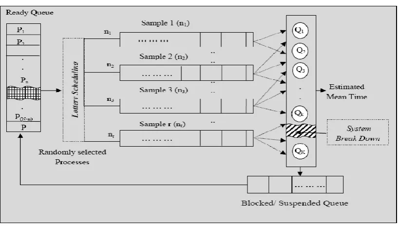
. When a process is blocked or suspended or interrupted, it is placed back to the respective queue [16]. The Figure 1 shows formation of different possible samples, through lottery scheduling of n processes from the ready queue, having pool of N processes, where k processors will get any sample of processes of varying sizes. Processes are processed completely or partially, before breakdown and processors generate time consumed in processing as denoted

j

y

(time by

th

[image:2.595.95.505.449.682.2]

j

processor) where



j



1 ,

2 ,

3 ,...,

k

,....

K



.

Figure 1. Lottery scheduling of processes to k processors with estimation of expected time after breakdown.

Other available information of processes is

i

x

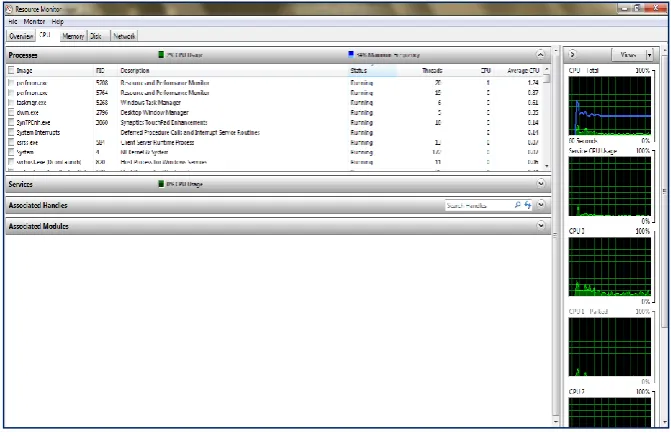
as a source of auxiliary variable. Figure 2 and Figure 3, shows

(3)

[image:3.595.129.465.72.290.2] [image:3.595.132.464.322.539.2]

Figure 2. Active processes in the system.

Figure 3. Processes with Disk Activity and Priorities.

4. ESTIMATION OF READY QUEUE

PROCESSING TIME (AS PER [17])

We know Ratio estimator:

 

r



02 11



... 1

 

B y



Y V



V

 

2





 

20

2

11 02

... 2

r

M y



Y

V



V



V

..(2)

Consider following notations;



1 ,

2 ,....,



0 ,









_i _i

i

d

X

x

i

N

where

z



d



X

Z





1 

1  

2 ;



A



d



d





1  

4 ;



B



d



d





2  

3  

4 ;



C



d



d



d



where

d

is a constant

(

0 

d





)

. Transformed

Factor-Type (T-F-T) estimator in [18] for Y , is









... 3

 

TFT

A

C Z

fBz

T

y

A

fB Z

Cz









_

_























 

1 (

)

... 4

1 A

C d

X

fB dX

x

y

A

fB d

X C dX

x



_

_

_

_



 



















Consider the large sample approximation



1 e

0



,

x

X



1 e

1



Y

y









, so that

 

e

₀



E

 

e

₁



0 ,

(4)

 

e

₀

e

₁



V

,

i

,

j



0 ,

1 ,

2 .

E

i j _ij

In above expressions





 





/

;

,



0 

E

y

Y

x

X

Y

X

Y

X

V

_ij i j i j …(5)



V



C

Y

C

X

V



₁₁

/

₀₂





/

Using notation Bias () for bias and M.S.E () for mean squared error, since the term





1 

1







fB

C

d

A

Ce

for our choice of A, B and C; We get the following expressions



T



Y



Q



1

V

02

V

11





Bias

_TFT













02 11



2 20

2

2 .

.

S

E

T

Y

V

Q

V

QV

M

_TFT





where

Q





₁





₂









1 

1



_

_

d

C

fB

A

C











1 

2







d

C

fB

A

fB



4.1. Suggested Ready Queue Processing

Time Estimators With Numerical

Illustration

Using[14] and [15], we suggest the two estimators as below;

At

_d



₅

, we choose one method from class

TFT

T

marked as A

T

,









 

72

20

4 ... 6

90

20

1

A

f X

fx

T

y

X

f

x











_

_









 

_

_{ }

_

02 11

 

3

2

3 ... 7

4 9 2

A

f

Bias T

Y

V

f



_



_



_







_



_





























 

2 20 02 2 11

3

2 4 9

2 . . (

)

... 8

3

2

2 4 9

2

A

f

V

f

M S E T

Y

f

V

f



_

_

_





_{ }

_

_







_

_





_

_











 







_

_



_







Similarly, at

d



6

, we choose another method in class

TFT

T

marked as

B

T







122

110

30

25 

12

5 ... 9

 

B

f

X

fx

T

y

f

X

x











_

_









 

_

_{ }

_

02 11

 

12

5

12 ... 10

5 22

5 5 22

5

B

f

Bi a s T

Y

V

f



_



_



_







_



_





























 

2 20 02 2 11

12

5 5 22

5 . . (

)

... 11

12

5

2 5 22

5

B

f

V

f

M S E T

Y

f

V

f



_

_

_





_{ }

_

_







_

_





_

_



_







 





_

_

_











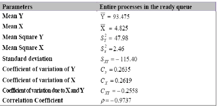
[image:4.595.122.486.569.748.2]

We assume that (N = 40) processes in the ready queue at a time in the system and n processes are currently running in the system at a time, whose snap shot of the CPU burst/usage time in seconds as Y and priority values as X is mentioned against them, displayed in Appendix A. The process population parameters are shown in Table 1.

(5)

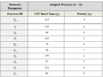
Suppose out of N processes, n are processed ( n < N ) and remaining (N - n) are still in the system unprocessed, when sudden disaster/collapse occurs. As an example Table 2, Table

[image:5.595.117.485.141.245.2]

3 and Table 4 shows samples of n (n = 5, 10, 15) processed processes before breakdown.

Table 2. Description of first sample n = 5.

[image:5.595.128.477.281.540.2]

(6)

Table 4. Description of third sample n = 15.

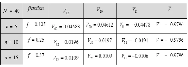
[image:6.595.138.468.579.696.2]

The table 5, shows the ready queue process parameters for the first sample (n = 5), second sample (n = 10) and the third sample (n = 15) (from Appendix A).

(7)

5. PERFORMANCE MEASURES OF

_T

_TFT

(AS PER [18])

An estimator is said to be more efficient estimator of the parameter (i.e. ready queue length prediction) than the other provided that it produces lower M.S.E values and

hence lower values of variances than the other one. Table 6, Table 7 and Table 8 presents numerical comparisons between the two estimators in terms of Bias and M.S.E.

Table 6. Bias and M.S.E comparison of

A

T

and

B

T

estimators (when n = 5).

The M.S.E ( = 328.39) and hence Variance ( = 328.25) of

B

T

is lesser than the M.S.E ( = 347.07) and Variance ( = 328.39) of

A

T

in above example Table 6 when n = 5.

A

T

and

B

T

Similarly, the M.S.E ( = 143.18) and hence Variance ( = 143.16) of

B

T

is lesser than the M.S.E ( = 151.40) and

Variance ( = 151.39) of

A

T

in above example Table 7 when n = 10.

A

T

and

B

T

Again it has been observed that the M.S.E ( = 80.84) and Variance ( = 80.83) of

B

T

is lesser than the M.S.E ( = 85.52) and Variance ( = 85.52) of

A

T

in above example Table 8 when n = 15. It has been observed that the estimator

B

T

produces better prediction for any values of n.

The 95% confidence interval of the mean time estimate using

A

T

and

B

T

are:

 

1, 2

[

_A _A

]

0.95 ... 12

n

P T

t

_

V T







 

1,

[

_B _B

]

0.95 ... 13

n

P T

t

_

V T







where

 



 

2



 

. .

... 14

A A A

V T





_

M S E T



Bias T



_

 



 

2



 

. .

... 15

B

V T





_

M S E T

B



Bias T

B



_

More explicitly, one can write 95% confidence intervals for mean estimation as

 

1,

2

1,

[

]

0.95

A A A

n

A n

P T

t

V T

Y

T

t

V T



 





(8)

 

1,

2

1, 2

[

]

0.95

B B B

n

B n

P T

t

V T

Y

T

t

V T



 









where

2 , 1



n

t

is t-value at (n - 1) degree of freedom and at



-level of significance. The

A

T

,

T

_B are the sample based

estimates of ready queue processing time parameter

_Y

. The

t

values are shown in the Appendix B. The time estimates

A

T

,

T

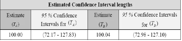
_B are predictors in the form of average time required

[image:8.595.131.469.234.312.2]

to complete a processes by processors using lottery scheduling. Table 9, Table 10 and Table 11 shows comparisons of the two time estimates and confidence intervals for the ready queue length in case of first sample (n = 5), second sample (n = 10) and third sample (n = 15) respectively.

Table 9. Confidence interval comparison of

A

T

and

B

T

A

T

and

B

[image:8.595.128.474.460.539.2]

T

A

T

and

B

T

These time estimates, hence confidence intervals as per Table 9 to11 shows that estimator

₍

₎

B

T

consistently produced narrow time intervals than estimator

₍

₎

A

T

.

So, the predicted total time required for processing remaining jobs in the ready queue using two methods are:

Remaining time estimate by





 

:

.... 16

A A A

t



N



n

T

Remaining

time

estimate

by

t

_B

:





... 17

 

B B

t



N



n

T

6. DISCUSSION AND CONCLUSION

This paper considers, two ready queue processing time estimation methods

A

T

and

B

T

which are mutually compared. In given examples the estimator

B

T

is uniformly

efficient over estimator

A

T

for n = 5, 10 and 15, as shown

in Table 9, Table 10 and Table 11 respectively (due to lower M.S.E). In each case, true values of CPU burst time lies within the range of confidence intervals when we use (T-F-T) estimator.

Incorporation of lottery scheduling in ready queue processing time estimate guarantees equal chance of selection of processes to the processor, to avoid starvation. The proposed estimators may be incorporated in practical utility programs for performance analysis or billing purpose. So, it is recommended to prefer

B

T

over

A

(9)

7. REFERENCES

[1] A.C. Waldspurger, E.W. Weihl, “Lottery Scheduling a flexible proportional-share resource management”, Proceedings of the 1st USENIX Symposium on Operating Systems Design and Implementation (OSDI), pp.1-11,1994.

[2] D. Petro, A.G. Gibson, W.J. Milford, “Implementing Lottery Scheduling: Matching the specializations in Traditional Schedulers”, Proceedings of the USENIX Annual Technical Conference USA, pp.66-80, 1999. [3] D. Yiping, F. William, “Interpreting Windows NT

Processor Queue Length Measurements”, Proceedings of the 31st Computer Measurement Group Conference, Vol.

[4] A. Tanenbaum, Operating System, Ed. 8, Prentice Hall of India, New Delhi, 2000.

[5] A. Silberschatz, P. Galvin, Operating System Concepts, Ed.5, John Wiley and Sons (Asia), Inc, 1999.

[6] Cochran, Sampling Technique, Wiley Eastern Publication, New Delhi, 2005.

[7] D. Singh, F.S. Choudhary, Theory and Analysis of Sample Survey and Designs, Wiley Eastern Limited, New Delhi, 1986.

[8] D. Shukla, A. Jain, A. Chowdhary, ” Estimation of ready queue processing time under Usual Lottery Scheduling (ULS) scheme in multiprocessor environment”, Journal of Applied Computer Science and Mathematics (JACSM), Vol. 11, no. 11, pp.58-63, 2011.

[9] D. Shukla, A. Jain, “Estimation of ready queue processing time under SL-Scheduling scheme in multiprocessor environment”, International Journal of Computer Science and Security (IJCSS), Vol. 4(1), pp. 74-81, 2010.

[10] D. Shukla, A. Jain, A. Chowdhary,” Estimation of ready queue processing time under Usual Group Lottery Scheduling (GLS) scheme in multiprocessor environment”, International Journal of Computer and Applications (IJCA), Vol. 8, no. 14, pp. 39-45, 2010. [11] D. Raz, B. Itzahak, H. Levy, “Classes, Priorities and

Fairness in Queuing Systems”, Research report, Rutgers University, 2004.

[12] D. Shukla, A. Jain, “Analysis of ready queue processing time under PPS-LS and SRS-LS scheme in multiprocessing environment”, GESJ: Computer Science and Telecommunication, Vol.33, no.1, pp. 54-61, 2012. [13] D. Shukla, A. Jain, “Estimation of ready queue

processing time using Efficient Factor -Type (E-F-T) estimator in multiprocessor environment”, International Journal of Computer and Applications (IJCA), Vol. 48, no. 16, pp. 20-27, 2012.

[14] V.K. Singh, D. Shukla, ”One parameter family of factor type ratio estimators”, METRON International Journal of Statistics, Vol. XLV- no. 1-2, pp. 273-283, 1987. [15] V.K. Singh, D. Shukla,”An efficient one-parameter

family of factor-type estimator in sample surveys”, METRON International Journal of Statistics, Vol. XVV, pp.139-159, 1992.

[16] W. Stalling, Operating Systems, Ed.5, Pearson Education, Singapore, Indian Edition, New Delhi, 2004. [17] T. Srivenkataramana, “A dual to ratio estimator in

sample survey”, Biometrika, Vol. 67, pp. 199-204, 1980. [18] D. Shukla, V.K. Singh, G.N. Singh, “On the use of