Munich Personal RePEc Archive
Real Exchange Rate Dynamics With
Endogenous Distribution Costs
Mulraine, Millan L. B.
September 2006
Online at
https://mpra.ub.uni-muenchen.de/9/
Real Exchange Rate Dynamics With Endogenous
Distribution Costs
∗(
Job Market Paper
)
Millan L. B. Mulraine†
September 2006
Abstract
The importance of distribution costs in generating the deviations from the law of one price
has been well documented. In this paper we show that a two-country flexible price
dy-namic general equilibrium model driven by exogenous innovations to technology, and with a localized distribution services sector can replicate the key dynamic features of the real
exchange rate. In doing so, the paper identifies the importance of two key channels for real
exchange rate dynamics. That is, we show: (i) that shocks in the real sector are important
contributors to movements in the real exchange rate, and (ii) that the endogenous wedge
created by distribution costs of traded goods is a significant source of fluctuation for the
real exchange rate, and the overall macro-economy as a whole. The evidence presented
here demonstrates that this model - without any nominal rigidities, can account for up to
89% of the relative volatility in the real exchange rate.
Keywords: Distribution costs, Real exchange rate dynamics, Law of one price.
JEL Classification: E31, F31, F41
∗This paper forms part of my Ph.D. Economics thesis at the University of Toronto. I wish to thank
G. Kambourov for his supervision of this effort, and the many others who offered helpful suggestions and
comments. All remaining errors are mine.
†Corresponding address: Department of Economics, University of Toronto, 150 St. George Street,
1
Introduction
In the international macroeconomics literature one puzzle remains as elusive today as it has been since its emergence thirty years ago - namely, the inability of theoretical economic models to replicate the key empirical features of the real exchange rate. That is, since the beginning of the post-Bretton Wood flexible exchange rate period of 1971, nominal and real exchange rates have exhibited significant volatility and persistence, and have been considerably more variable than the underlying economic fundamentals assumed to be associated with their determination. Following the publication of Dornbusch (1976) ‘overshooting’ model1, the
quest of the new open economy macroeconomics literature has been to explain this puzzling behavior of bilateral real exchange rates by means of dynamic general equilibrium monetary models with nominal rigidities in the form of sticky prices, `alaObstfeld and Rogoff(1995).
This literature was further advanced by the monopolistic pricing-to-market model devel-oped by Betts and Devereux (1996), which took account of the well established empirical observations on the pronounced deviations from the law of one price in traded goods - see
Lane (2001) for a survey of the new open economy literature. This particular approach, however, is predicated on the assumption that movements in the deviation in the law of one price is due to rigidities in the pricing structure for these goods and not the wedge created by the distribution costs of these goods. Moreover, the fundamental premise of this strand of the literature is that the dynamic behavior of the exchange rate is due to the interaction between shocks to the money supply and sticky prices - thereby obviating the role of produc-tivity innovations in determining the behavior of the real exchange rate, as postulated by the Balassa-Samuelson proposition2.
In an attempt to offer quantitative justifications for this approach, Chari et al. (2002) constructs a monetary dynamic general equilibrium (DGE) model to show that a model with
1
In this elegant theoretical exposition it was shown that the volatile behavior of the exchange rate was
consistent with rational expectations in the presence of price rigidities. The overshooting of the nominal
exchange rate beyond its long-run level, therefore, was shown to be the results of the interaction between
monetary shocks and sluggish price adjustment.
2
The Balassa-Samuelson hypothesis, due to the work ofBalassa(1964) andSamuelson(1964), asserts that
an increase in the productivity of tradables relative to non-tradables in the home country, if larger than the
price stickiness for at least one period, and high risk aversion can replicate the fluctuations in the real exchange rate between the US and a European aggregate. They also show that adding real shocks (in the form total factor productivity (TFP) and government spending shocks) to their stylized model “change the model predictions little” - thereby concluding that real shocks are not important in explaining the dynamics of the real exchange rate.
The empirical evidence on the dynamic behavior of the real exchange rate over the post-Bretton Wood floating exchange rate period, however, casts doubts on the importance of shocks to the money supply in explaining the deviation in the real exchange rate. Alexius
(2005) shows that between 60-90% of the volatility of the real exchange rate can be accounted for by relative productivity shocks across trading partners, thereby providing evidence that confirms the long held view of a Balassa-Samuelson effect on the real exchange rate. In addition to this study, Carr and Floyd (2002) shows that the dynamic behavior of the US-Canada real exchange rate, for example, can be explained by asymmetric real shocks, and that there appears to be no evidence to support the view that monetary shocks have had any significant impact on the dynamic behavior of the real exchange rate. Despite this evidence, the use of real quantitative general equilibrium models to explain the dynamic behavior of the real exchange rate has been largely absent from the international macroeconomics literature. In this paper, we present evidence that confirms the Balassa-Samuelson proposition by positing a real DGE model with a localized distribution services sector, and in so doing provide an avenue for this strand of the literature to be further advanced.
domestically available consumer good. Thus, the model endogenously generates the wedge between the price of traded goods between the two countries, as observed in the data. The standard approach in the literature has been to assume that the consumption of a unit of imported consumer good requires a fixed amount of distribution services.
In this paper we develop a stylized two-country DGE model driven solely by exogenous innovations to real factors in the economy to demonstrate that this model can replicate the dy-namic behavior observed in the real exchange rate between the US and a European aggregate. In particular, we specify a non-monetary DGE model driven by shocks to investment-specific technology (IST) and with a localized distribution services sector to show that a stylized model without nominal rigidities can match the stylized facts of the real exchange rate. The inclusion of a distribution service sector enables us to endogenously generate the deviations from the law of one price which has been a key feature of the real exchange rate and thus accounts for the contribution of the volatility in the real exchange rate made by movements in the relative price of traded goods.
The main exogenous propagation mechanism considered in this paper is shocks to the efficiency in the production of next period’s capital goods - or investment-specific technology shocks. To take account of this unique measure of productivity innovation investment in machinery and equipment - which is a tradeable good - is directly affected by improved efficiency in their production of next period’s capital stock. This form of innovation was shown by Greenwood et al. (1988, 2000) to account for over 30% of output fluctuation in the postwar US data. Further evidence on the impact of innovations to relative prices on the business cycle behavior of the US economy has been provided by Fisher (2003), who -using more recent data - finds that investment-specific technology shocks can accounts for over 50% of business cycle variation in hours worked, compared to only 6% accounted for by shocks to total factor productivity. Boileau (2002) also uses this propagation mechanism in a two-country framework to explore its ability to explain the cross-country correlation of output and the terms of trade.3 As a comparison to the dynamics generated by the model
propagated by investment-specific shocks, we shall also simulate the model using shocks to TFP.
3
Letendre and Luo(2005) andMulraine(2004) also use this propagation mechanism in an open economy
In more recent work,Jin and Zeng(2005) develops a flexible price model with distribution costs to show that with reasonably large distribution costs their model can generate highly volatile and persistent real exchange rate. This paper, however, differs from their work in a number of key dimensions. In this paper the innovation considered in this stylized economy comes from shocks to the efficiency of investment goods and not the Solow-neutral total factor productivity shocks considered in their work. Their model also incorporates innovations to the money supply. Secondly, and more importantly, in this paper we consider a distribution services sector instead of assuming that distribution costs are a fixed proportion of the price of traded consumer goods. And finally, in the model presented here, countries trade in not only consumption goods - as considered in their work, but also in the intermediate capital good.
The remainder of the paper proceeds as follows. In Section 2 of this paper the model is presented with its dynamic features discussed in Section3. In Section 4the model solution is discussed and the simulation results from the calibration of the model to match the stylized facts of the real exchange rate presented. The paper then concludes in Section5.
2
The Model Environment
Consider a two-country, multi-sector general equilibrium open economy model in which each economy is comprised of three types of agents; a representative consumer, a representative consumer goods producer, and a representative distribution services firm. The two economies considered are structurally symmetric, as such it will suffice to describe the agents and their activities in the home country, with an asterisk (*) denoting variables associated with the foreign country. These two economies are connected to each other through their trade in intermediate capital goods, consumer goods and financial assets.
2.1 The Representative Consumer
Each economy is populated by a large number of infinitely-lived identical agents of mass one who has taste for both domestic c1t and foreign produced consumer goodscm1t. Each period
servicesldt. Labor is considered to be perfectly mobile across two productive sectors, but will
be completely immobile across the two economies. The representative consumer chooses consumptionct to maximize their expected discounted utility function expressed by:
E0
∞
X
t=0
βtlog(ct), 0< β <1 (1)
wherect is the consumption level of the composite consumer good which comprises of home
and imported final consumption goods. The composite consumption goodctis such that:
ct=G(c1t, cm1t) (2)
where we aggregate home produced c1t and imported cm1t final consumption goods using a
constant elasticity of substitution (CES) aggregator functionG(c1t, cm1t) given by:
G(c1t, cm1t) = [ωc(c1t)ηc+ (1−ωc)(cm1t)ηc] 1
ηc (3)
This functional form of the CES aggregator enables us to characterize the respective prefer-ences for home goods (or home bias) given by ωc relative to imported consumption goods,
and the constant elasticity of substitution between home and foreign produced final goods,
σc = 1−1ηc.
The representative household has access to a perfectly competitive international capital market where they can trade in international financial assets at at the endogenously
deter-mined risk-free world interest rate rt. The accumulation of this type of financial asset will
evolve according to the following process:
at+1 =tbt+ (1 +rt)at (4)
wheretbt is the trade balance for the given period.
Each period, after observing the productivity innovation, the representative consumer devotesit of the total income in the form of investment which is used towards the creation of
intermediate capital goods. This shock represents an exogenous innovationqtto the efficiency
of this investment good4 in the creation of the total domestic stock of intermediate capital
4Following the work ofGreenwood et al.(2000), this paper espouses the use of
capital-embodiedtechnological
changes as the main contributor to economic fluctuations in the economy considered. For an elaborate and
exhaustive discussion on the issues related to the use of shocks to the efficiency of investment goods as a
goods given bymt=qtit. This stock of domestic intermediate goods is then divided between
the portion used domestically k1t for the production of next period capital stock, and the
portion that is exportedk∗1tsuch that,mt=k1t+k∗1t. The total domestic gross investment in
the capital stock for the current periodxt involves a combination of domestick1tand foreign
(imported) intermediate capital goodsk2t. Such that:
xt=H(k1t, k2t) (5)
where we aggregate home and foreign intermediate goods using a constant elasticity of sub-stitution (CES) aggregator functionH(k1t, k2t), such that:
H(k1t, k2t) = [ωk(k1t)ηk+ (1−ωk)(k2t)ηk] 1
ηk (6)
Similar to the composite consumption goods outlined above, this functional for the interme-diate good aggregator characterizes the respective preference for home goods (or home bias) given byωkrelative to foreign goods, and the constant elasticity of substitution between home
and foreign produced final goods,σk= 1−1ηk.
The representative consumer purchases the output of the consumer goods firmytand the
output of the distribution goods firmcm
1t from the available income for that period. In
addi-tion to trade in the intermediate capital goods, the consumer exports domestically produced consumer goods c∗
1t and trades in foreign assets at. As such, the budget constraint for the
representative consumer is given by:
c1t+pm1tcm1t+pktk1t+p∗ktk2t+tbt+
φa
2
(at+1−¯a)2≤wt+rtkt (7)
Subject to the following function which captures the evolution of the capital stock - net of the capital adjustment costs:
kt+1 = (1−δ)kt+xt−
φk
2
(kt+1−kt)2 (8)
Where the variablextcaptures the stock of intermediate goods added to the non-depreciated
as the cost(s) associated with the installation of new machinery and equipment. This cost could be considered to include training, installation fees and the cost of disposing of the old stock of machinery. The essential thing to note here, however, is that this cost will act as a moderating force on the investment decision of domestic agents, thereby eliminating excessive responsiveness in investment decisions to small rate differentials and to ensure that any adjustment to the capital stock is gradual.
Following Schmitt-Groh´e and Uribe (2003), we introduce a convex portfolio adjustment cost given by
φa
2
(at+1−¯a)2 to prevent agents from playing Ponzi-type games, and
conse-quently ensuring stationarity in the behavior of net foreign asset holdings. In this framework, given the symmetric nature of the two economies considered the steady-state value of net foreign asset is assume to be zero, that is (¯a= 0).
2.2 The Representative Final Goods Firm
The home country produces an internationally tradeable composite consumption commodity whose Cobb-Douglas production technology is given by:
yt=ztkαctlct1−α (9)
Wherezt, kct and lct represent the innovation to total factor productivity in the production
of consumer goods, and the amount of capital and labor services which are allocated to this sector, respectively. Thus, the static profit maximization problem for this representative consumption good producer in the home country is given by:
maxπtc =yt−wtlct−rtkct (10)
Note that the constant returns to scale technology for this consumptions goods firm necessi-tates that it makes zero profit.
2.3 The Localized Distribution Sector Firm
of this expenditure are housing, health and education services. This representative distri-bution sector firm, therefore, provides all the requisite services that are entangled in the movement of the imported consumption goodsc2t from its ‘point of entry’ in the home
econ-omy to the ‘point of consumption’ cm
1t. These services include transportation, advertising,
insurance, warehousing and all other services associated with bringing the imported goods from the border to the retail outlet. In accordance with the findings ofBurstein et al.(2004), we abstract from having traded investment goods requiring any distribution services, since they have shown that the share of distribution services in the retail prices of investment good is very low. As a result, the profit maximization problem for this sector is given by:
maxπtd=pm1tcm1t−wtldt−rtkdt−p2tc2t (11)
subject to a Cobb-Douglas production function given by:
cm
1t= [ωd(dt)ηd+ (1−ωd)(c2t)ηd] 1
ηd (12)
In this regard, the distribution firm takes the imported consumer goods c2t and augments it
with distribution services dt before making it available at the consumer outlet as cm1t. The
production function for the distribution service is given by the following function:
dt=ztkdtαldt1−α (13)
One key feature of this framework is the fact that the distribution cost associated with the movement of the imported consumer good from the border to domestic consumers in this model φd
t = pm1t−p2t arises endogenously, a departure from the standard literature where
these costs are considered to be fixed and exogenously. Note that the distribution firm pays
p2t at the border for the imported consumption good and sells it at pm1t to home consumers.
The constant returns to scale technology for the representative distribution services firm ensures that profits are zero, and consequently the retail price of the imported consumer good includes no mark-up. As before, the functional for the imported good aggregator characterizes the respective share of the imported good accounted for by distribution services given byωd
2.4 The Real Exchange Rate
To assess the dynamic properties of the real exchange rate of this stylized model we shall use two definitions of the real exchange rate. The first of which will be the real exchange associated with consumer prices. Recall that the representative consumer in both economies consumes two types of consumer goods - domestically produced consumer goods and the imported consumer good - given byc1t and cm1t, respectively, for the domestic consumer, and
c2t and cm2t for the foreign consumer. The prices associated with these commodities are p1t
(normalized to 1) andpm
1t, for the domestic consumer andp2tandpm2tfor the foreign consumer.
As such, given that the CES functional form of the utility function, the CPI for the home countrypc
t and the foreign economyp c,∗
t are given by:
pct = hω
1 1−ηc
c + (1−ωc) 1 1−ηc(pm
1t)
ηc ηc−1
iηc−1 ηc
(14)
pc,t∗ = hω
1 1−ηc
c (p2t)
ηc
ηc−1 + (1−ω c)
1 1−ηc(pm
2t)
ηc ηc−1
iηc−1 ηc
(15) If the law of one price for the traded consumer goods were to hold, then we would expect the consumer price of the traded consumer goods to be such thatp2t=pm1t and p1t =pm2t =
1. Following Betts and Kehoe (2001), we obtain an expression for the real exchange rate associated with consumer prices as:
rerc t =
pc,t∗ pc
t
(16) Similarly, we can derive the the real exchange associated with the intermediate capital good - based on producer prices. Recall that the representative consumer in both economies uses two types of intermediate capital goods in the production of next period’s capital goods - domestically produced investment good and the imported investment good - given by k1t
and k2t, respectively for the home consumer, and k2t∗ and k1t∗ for the foreign consumer. The
prices associated with these commodities arepktand p∗kt, for the domestic consumer and p∗kt
andpktfor the foreign consumer. As such, given that the CES functional form of investment,
the PPI for the home countrypk
t and the foreign economyp k,∗
t are given by:
pkt = hω
1 1−ηk k (pkt)
ηk
ηk−1 + (1−ω k)
1 1−η(p∗
kt)
η η−1
iηk−
1
ηk (17)
pk,t∗ = hω
1 1−ηk k (p
∗
kt)
ηk
ηk−1 + (1−ω k)
1 1−ηk(p
kt)
ηk ηk−1
iηk
−1
ηk
We obtain an expression for the real exchange rate associated with producer prices as:
rerkt = p
k,∗
t
pk t
(19)
2.5 Stochastic Processes
To close the model setup the propagation mechanism for the shocks to IST and TFP are described by the following processes:
qt+1 = Γqqt+ξqt (20)
and
zt+1 = Γzzt+ξtz (21)
Where q = [ln(q),ln(q∗)]′ and z = [ln(z),ln(z∗)]′ . Here Γ
q and Γz are the matrices of
coefficients, andξq andξz are the vectors of mean zero normal random variables with
contem-poraneous variance-covariance matrix given by Σq and Σz, corresponding to the innovations
to IST and TFP, respectively.
2.6 Model Behavior
In order to provide intuition into the model’s behavior we shall briefly analyze the main channels of operation present. Recall that the dynamic behavior of this model hinges on two key features incorporated in this framework, namely: (i) the distribution services sector, and (ii) trade in both consumer and intermediate capital goods. The first of these features provides the natural wedge between the domestic and foreign price of traded consumption goods - or the deviation from the law of one price in traded goods. This endogenous wedge arises from the fact that imported consumption goods must first be augmented with domestic distribution services before they are consumed by agents in the model.
price index of the respective economies. The endogenous nature of this sector means that this wedge will vary with relative prices, and will not be constant as is the standard in the literature. Moreover, because distribution services require the input of labor and capital, there is an inevitable trade-off between the production of domestic consumer goods and distribution services.
The trade in both producer and consumer goods - with only consumer goods requiring distribution services, provides another key conduit through which any propagation can have divergent impacts across the two economies. Foremost among these will be its impact on the consumption and investment decision of agents during the period in which the shock occurs. Because the final consumptionctand investment xt good requires a mix of domestic
and foreign produced goods, and with the elasticity of substitution between these goods being constant, there will be opportunities for technology and wealth sharing across the two economies as a result of asymmetric shocks.
For example, consider a unit shock to investment efficiency in the domestic economy relative to the foreign economy. The first-period wealth effect from this innovation will result in increased consumption and investment for domestic agents, while the substitution effect will favor accumulation of investment goods relative to consumption goods. The decrease in consumption will favor the importation of the relatively cheaper foreign-produced consumer goods while the increase in capital will result in the creation of more domestic intermediate capital goods. To finance these additional expenditure, domestic agents will inevitably borrow against the higher rate of return from capital in the future. Clearly, the ramifications of these two effects cannot be fully analyzed in this stochastic model as they will affect not only the quantities traded, but also the prices of these commodities traded and consequently, the aggregate price level. As a result we shall now turn to the numerical solution to the model.
3
Recursive Problem for the Home Economy
Let V(k, k∗, a, q, q∗, z, z∗) be the value function for the representative agent whose assets at the beginning of the period are given by the holding of foreign assets a, and the stock of capital k, and who faces the equilibrium wage and rental rate of capital are given byw and
described byλ(k, k∗, a, q, q∗, z, z∗), where A(λ) andK(λ) are the aggregate holding of assets, andP(λ),R(λ), andW(λ) are the aggregate vector of prices, and the equilibrium rental price for capital and labor, respectively. The dynamic problem facing the representative household of the home economy5 who takes the aggregate state of the world as given can be represented
by the following Bellman equation:
V(k, k∗, a, q, q∗, z, z∗) = max
a′,c
1,cm1,c2,k1,k2,k′,kc,lc
{log(c) +βE[V(k′, k∗′, a′, q′, q∗′, z, z∗′)]} (22) subject to:
c1+p2c2+pkk1+p∗kk2+tb+
φa
2
(a′−a¯)2 ≤y+d (23)
tb=a′−(1 +r)a (24)
lc+ld≤1 (25)
kc+kd≤k (26)
k′ = (1−δ)k+x−
φk
2
(k′−k)2 (27)
x= [ωk(k1)ηk+ (1−ωk)(k2)ηk] 1
ηk (28)
c= [ωc(c1)ηc+ (1−ωc)(cm1 )ηc] 1
ηc (29)
cm1 = [ωd(d)ηd+ (1−ωd)(c2)ηd] 1
ηd (30)
y =zkα
cl1c−α (31)
d=zkαdl1d−α (32)
q′ =ρqq+ρq,q∗q∗+εq (33)
and
z′ =ρzz+ρz,z∗z∗+εz (34) 5
3.1 Definition of the Competitive Equilibrium
A competitive equilibrium for the decentralized world economy is a vector of prices P(pm 1 ,
pm
2 ,p2,pk,p∗k,r,w w∗)6 and allocations (a′,k′,c1,cm1 ,c2,k1,k2,kc,kd,lc,ld) for the home
country, and (k∗′,c∗1,cm
2 ,c∗2,k1∗,k2∗,kc∗,kd∗,l∗c,ld∗) for the foreign country such that:
1. The representative households in the home and foreign country solve their problems taking the aggregate state of the worldλ(.) and the vector of aggregate pricesP(.) as given, with the optimal allocations to their problem satisfyinga′ =A′(λ), c
1 =C1(λ), c∗1 =C1∗(λ),
cm
1 = C1m(λ), cm2 = C2m(λ), k1 = K1(λ), k∗1 = K1∗(λ), k2 = K2(λ), k∗2 = K2∗(λ), k′ = K′(λ)
andk∗′
=K∗′
(λ);
2. Given prices, the allocations lc = Lc(λ), l∗c = L∗c(λ), kc = Kc(λ) and kc∗ = Kc∗(λ),
solve the profit maximization problems for the representative consumer goods producers in the home and foreign economy.
3. Given prices, the quantities c2 = C2(λ), c∗2 = C2∗(λ), ld = Ld(λ), ld∗ = L∗d(λ),
kd = Kd(λ) and k∗d = Kd∗(λ) solves the profit maximization problems for the
representa-tive distribution services firms in the home and foreign economy. 4. All factors and goods markets clear.
5. The global goods and asset markets7 clear. Such that:
tb+tb∗ = 0 (35)
4
Quantitative Assessment
Having fully specified the model, we shall now turn to the quantitative assessment of its properties. Note that due to the stochastic nature of the model specification, the competitive equilibrium allocations do not have closed-form analytical solutions. Thus, the model must be solved numerically. This will be done by finding an approximate solution to the log-linear
6
All prices considered in this model economy are expressed relative to the price of the domestically produced
consumer goodp1 - which has been normalized to 1. As such, the relative price of the traded intermediate
goodsk1 for the home country andk2 for the foreign country, are given bypk=1q andp∗k= p2
q∗, respectively.
Note that these prices correspond to the relative price of investment goods in the respective economies.
7
The trade balance (or net exports) for the home economy is given by tb=c∗1+pkk1∗−p2c2−p∗kk1. As
approximation of the first order conditions about their steady-state values. The approach used here is akin to the method advocated byKing et al. (1988), and is similar to that used by Schmitt-Groh´e and Uribe (2003). A complete discussion of the solution to this model, and the derivation of its steady-state properties is provided in Appendix A.1 - A.3 of the paper. The moments used in this analysis are the relative percentage standard deviation -that is, the standard deviations of the macroeconomics variables of interest relative to the standard deviation of GDP, the first-order autocorrelation of each variable of interest, and their respective cross-country correlation.
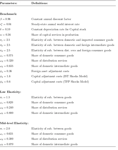
4.1 Parameter Calibration
Since the two economies considered in this framework are symmetric in all respects, all the parameters used have the same value in both economies. SeeTable 3for a complete summary of all parameter values. FollowingBackus et al. (1994), the constant discount factor is set at
β= 0.96, corresponding to an annual steady-state interest rate ofr∗ = 0.04, and the constant depreciation rate for capital was set at δ = 0.10. For the benchmark model the value of the elasticity of substitution between home and foreign consumer goods, distribution services and imported consumer goods, and home and foreign machinery and equipment were set to
σc = σd = σk = 2.5, such that ηc = ηd = ηk = 3/5, respectively. To determine the share
parameters for the domestic consumption goods, investment goods and distribution services given by, ωc, ωk and ωd, respectively, we follow the calibration procedure of Boileau (2002)
who set the steady-state output share of trade in final goods and trade in equipment to 20% and 10%, respectively. In addition to these output shares, following the findings of Burstein et al. (2003), we also set the steady-state distribution margin for imported consumer goods equal to 42% - equivalent to the distribution margin for consumer prices in the US. As a result of this calibration procedure, we obtain the respective shares given byωc= 0.575,ωk= 0.635
andωd= 0.320.
would expect the price deviation across countries to be lower, given the inverse relationship between the elasticity of substitution and the terms of trade. Consequently, this high value will provide us with the lower limit on the volatility of the real exchange rate in this framework.8 FollowingBoileau (2002), the productivity innovation to investment efficiency has a stan-dard deviation of 0.013 and a cross-country correlation of 0.345. The exogenous investment-specific shock process has a autocorrelation of 0.553 and a cross-country feedback of 0.027. As such the matrices for Σq and Γq are given by.
Σq= 10
−4
1.687 0.582 0.582 1.687
, Γq=
0.553 0.027 0.027 0.553
For the properties of the innovation to TFP we follow Kehoe and Perri(2002) andChari et al.(2002), in which case the standard deviation is set at 0.007 and a cross-country correla-tion of 0. The zero cross-country spillover follows the findings ofBaxter(1995) andKollmann
(1996) who find very little evidence of technology spillover. The exogenous investment-specific shock process has a autocorrelation of 0.95 and a cross-country feedback of 0.025. As such the matrices for Σz and Γz are given by.
Σz= 10
−4
0.4900 0.1125 0.1225 0.4900
, Γz=
0.95 0 0 0.95
Given the parameter values for the stochastic processes described above, the only remain-ing parameter to be determined in this model will be φi, i∈ {a, k} - the adjustment costs
parameter. These parameter are particularly important since they determine (to a large ex-tent) the investment and net foreign assets responses to innovations to the exogenous process considered. Despite their significance, however, these parameters cannot be determined ex-ante as they have no empirical counterparts. As such, we set their values in a manner that will limit the volatility in investment, while simultaneously ensuring stationarity in all macroeco-nomic variables. In particular, we set them such that the volatility of consumption is equal to its empirical counterpart and to ensure stationarity in the holding of net foreign assets. To this end, we use a value of φa = 0.36 and φk = 1.60. This value of the capital adjustment
cost is close to the lower limit of the range of 1.50 and 2.32 advocated byGreenwood et al. 8
(2000). For the TFP shocks model we followKehoe and Perri (2002) by setting the capital adjustment cost parameterφk= 0.60.
4.2 Simulation Results
This section is primarily aimed at comparing the performance of the model presented in matching the dynamic properties of the data. To do this, particular attention will be paid to the ability of the model to match key moments in the data. That is, we shall examine the percentage standard deviation (relative volatility)9, first-order autocorrelation and cross-country correlation of total consumption, total investment, net export, the CPI-based real exchange rate, and the PPI-based real exchange rate. Further analysis will be conducted by examining the associated dynamics of these variables of interest by studying the impulse responses generated from a 1% shocks to technology.
4.3 Investment-Specific Technology (IST) Shocks Model
The requisite unconditional moments generated from the simulation exercises are presented inTable 1below. Column 2 of Table 1refers to the associated moments obtained fromChari et al. (2002). In Columns 5 we present the unconditional moments for the macroeconomic aggregates for the benchmark model, in which case the elasticity of substitution between traded goods are set atσi = 2.5. As seen in this column, with the model simulated to match
the relative standard deviation of consumption, the model can explain as much as 32% of the CPI-based real exchange rate, with the relative volatility of the PPI-based real exchange rate being twice that of its CPI-based counterpart. The model also provides autocorrelation statistic for the CPI-real exchange rate that are relatively close to those observed in the data. The benchmark model matches quite reasonably the persistence of consumption and GDP, though it does a better job at matching the high persistence of consumption than it does in matching that of GDP. Despite the appealing performance in matching the relative volatility and persistence of the real exchange rate, consumption and GDP, the model performs very poorly in matching the empirical behavior of investment. As is evident for the table, the model overestimates the relative volatility of investment by a factor of 2 and underestimates
9
We do not directly report the volatility of the variables of interest but instead report their volatility relative
its persistence by a factor of 2. This excessive volatility emerges as a consequence of the high elasticity of substitution considered and is a direct consequence of the nature of the productivity innovation considered, similar to the evidence documented byBoileau (2002).
In terms of the cross-correlation of the macroeconomic aggregates, the benchmark model has been able to replicate the positive cross-correlation of GDP, consumption and investment - consistent with the data. This outcome is important since it highlights the fact that this model with trade in equipment avoids the counterfactual negative cross-country correlation in investment and almost-perfect cross-country correlation in consumption - two outcomes that have been the feature of standard international business cycle models. In essence, by incor-porating trade in equipment, the innovation to investment technology in the home country is exported to the foreign country which will invariably benefit from this new technology, consis-tent with the empirical observations. This feature mitigates against the impact of risk-sharing in form of financial asset flows to the country with the favorable productivity innovation, thereby eliminating the negative cross-country investment correlation and the associated high cross-country correlation of consumption.
In addition to these key features, the model is also able to correctly replicate the ranking of the cross-country correlation of output and consumption, compared to the standard pre-dictions in the literature. In general, stochastic DGE models have provided estimates of the cross-country correlation of consumption that have been higher than that of output, opposite to the observed ranking in the data where ρy,y∗ > ρc,c∗. This anomaly has been called the
“quantity puzzle” byBackus et al. (1992). This progress, however, must be tempered by the fact that these statistics are over-estimated by a factor of two, relative to the moments in the data in the case of consumption.
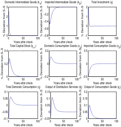
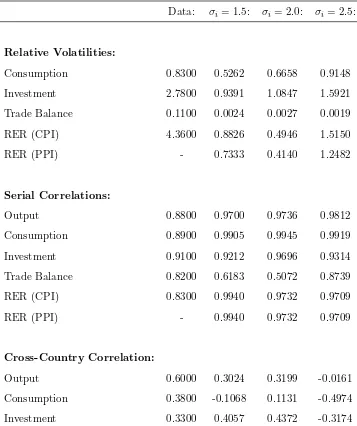
The dynamic behavior of the variables of interest in the stylized model following a 1% shock to investment-efficiency - with the elasticity of substitution set to 2.5 - are presented in
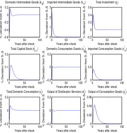
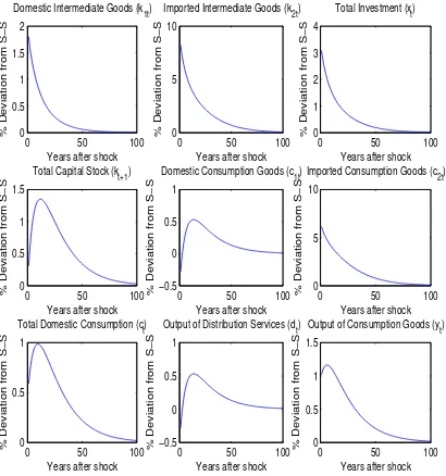
investment in the two countries, however, differs as the home country experiences a consider-ably higher increase in investment than its trading partner. Consistent with economic theory, the home country substitutes the foreign intermediate goods for the more efficient domestic counterpart, while in the foreign country the local intermediate goods was substituted by the relatively cheaper imported investment goods.
The behavior of total consumption in these two economies is also instructive. As is evident from the graph total consumption falls significantly in the first period before rising above its steady-state level in both countries. Similar to the evidence on the behavior of investment accumulation, the level of consumption falls by a larger amount in the foreign country than in the home economy. In the home country the substitution effect dominated the wealth effect from the higher productivity in the home country as agents substitutes consumption in the initial period of the shock for investment goods which was used to financed the higher consumption (relative to its steady-state level) in subsequent periods. Note that in the home country the greater increase in investment along with a smaller reduction in consumption relative to the foreign country was financed by the accumulation of foreign debts.
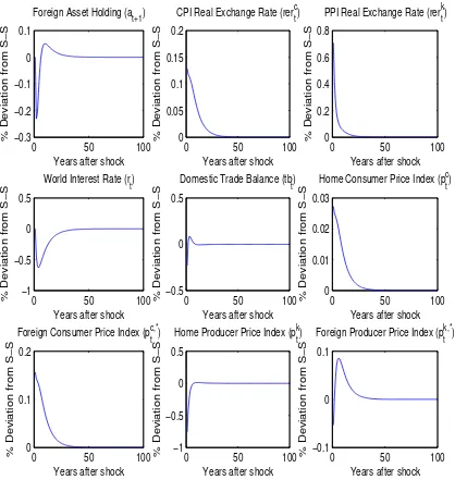
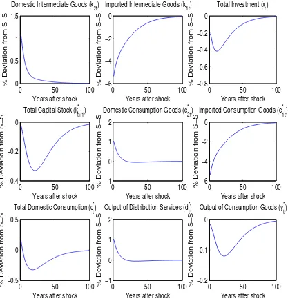
Figure 3provides dynamics for the various prices and the domestic holdings of net foreign assets. As seen, the home country accumulates foreign debts (negative trade balance) which is used to financed its increased investment and consumption over the horizon of the analysis. The dynamic movement of the price indices considered and their associated real exchange rate is consistent the Balassa-Samuelson, the productivity shock resulted in a depreciation in the real exchange rate.
4.4 The Role of the Distribution Sector
To ascertain the role of distribution services in generating the dynamics of the real exchange rate in the benchmark model, we posit a more parsimonious model with a modified localized distribution services sector. That is, we assume that the quantity of distribution services required to augment the foreign-produced imported consumer goods c2t in the production
of the locally consumed imported good cm
tradeable consumer goods10. That is:
dt=φdyt (36)
Whereφd was set equal to 0.02 to reflect the fact that in the steady-state of the benchmark
model distribution services accounted for 2% of GDP. Note that in this framework the cap-ital stock and the unitary supply of labor will be devoted entirely to the production of the tradeable consumer good. Moreover, for the sake of comparative purposes we maintained the parameterization used in the benchmark model. The results from this simulation exercise are presented in Column 6 ofTable 1 below.
From the results presented inTable 1it becomes evident that the modified model generates far less volatility than the benchmark model. In the case of the CPI-based real exchange rate we have that the relative volatility is almost ten times smaller than in the benchmark model, while for the PPI-based model the reduction in the volatility if by a factor of 3. The majority of this reduction arises from the reduced volatility in the domestic price of the traded consumer goodpm
1t11- a direct consequence of the reduced volatility of the distribution
costs. The disproportionate reduction in the relative volatility of the CPI-based real exchange rate compared to the relative volatility of the PPI-based real exchange rate results from the definition of the the CPI-based real exchange rate given by Equation 14 - 16, in which case it becomes evident that the endogenous wedge created by the distribution costs becomes less volatile thereby reducing the volatility of the domestic price of the traded consumer goodpm
1t.
The modified model configuration also resulted in reduced relative volatility in investment and the trade balance - with a modest increase in the relative volatility of in consumption. More generally, this model also correctly replicates the ranking of the cross-country corre-lation of output and consumption, consistent with the stylized fact. We also obtained, but do not report here, the impulse responses of the main macroeconomic variables of interest. These impulse responses are similar in their direction to the benchmark model with the main difference being that the magnitude of the responses were less than in the benchmark model - as expected.
10
All the other features of the benchmark model were maintained.
11Recall that the domestic price of the imported consumer good
pm
1t=p2t+φdt. Whereφdt is the distribution
4.5 Sensitivity Analysis
Following Backus et al. (1994), we vary the value of the elasticity of substitution as a sen-sitivity check of the behavior of the benchmark model. In Column 3 of Table 1 we provide unconditional moments for the macroeconomic aggregates for an elasticity of substitution equal given by σi = 1.5, and in Column 4 we provide moments for σi = 2.0.12 The values
for the adjustment cost parameters were maintained at the same level as in the benchmark model. Note also that to maintain the import shares outlined above, the CES shares given by theωi’s must also be re-calibrated. The re-calibrated values are provided in Table 3below.
The evidence provided in Table 1 shows that in the case of the IST shocks model, the lower the elasticity of substitution the better the performance of the model in matching the relative volatility of the CPI-based real exchange rate. In the case of the “low elasticity” case the model matches over 90% of the relative volatility of the CPI-based real exchange rate. The model also improves on matching the empirical properties of investment. In addition to slight improvements in the volatility of investment13, the model correctly replicates the stylized facts on the cross-country correlation of GDP, consumption and investment. That is, the evidence provided shows that a model with trade in equipment avoids the counterfactual negative cross-country correlation in investment and almost-perfect cross-country correlation in consumption obtained by the standard two-country real business cycles models. Moreover, the model was also able to achieve the cross-country correlation ranking of consumption and output observed in the data, thereby providing an avenue for solving the “quantity puzzle”.
4.6 Total Factor Productivity (TFP) Shocks Model
In Table 2 we present the simulated values for the unconditional moments of the stylized model propagated by innovations to TFP14. It is evident from this table that the standard
TFP shocks model performs very poorly in replicating the stylized features of the real exchange
12
The associated impulse responses for these values of the elasticity of substitution are not shown.
13
Note that the volatility of investment generated by the model remains three times the size observed in the
data.
14
The features of this TFP shocks model is identical to the IST shocks model considered above with two
exceptions. Firstly, the properties of the innovations to TFP were taken fromKehoe and Perri(2002) and
Chari et al.(2002). Secondly, the value for the capital adjustment costs parameter in this model was set equal
rate. As seen, this form of productivity innovation accounts for at most 35% of the relative volatility of the CPI-based real exchange rate, compared to the corresponding values of 89% from the IST shocks model. This outcome concurs with the findings of Chari et al. (2002) who show that adding real shocks (in the form TFP and government spending shocks) to their stylized model “change the model predictions little”. On the other hand, this model outperform the IST shocks model in matching the relative volatility of investment by obtaining estimate that are not as excessively volatile as in the IST shocks model.
The model also does poorly in matching the observed cross-country correlations of the macroeconomics variables of interest. In particular, the estimates of the benchmark model
σi = 2.5 exhibit negative cross-country correlations. This outcomes is the result of the
as-sumptions of zero spill-over in the TFP innovations across the two countries and the high elasticity of substitution between the goods. This feature of the model is in sync with similar estimates in the literature. The signs of the estimates, however, reverses when the elasticity of substitution is reduced - with the exception of consumption which remained negative in the low-elasticity case. In terms of the serial correlation of the variables, the estimates were reasonably close to their empirical counterpart with the serial correlation of investment being particularly close.
As a way of understanding the discrepancies in the behavior of the TFP shocks model we present impulse responses of some variables of interest to a 1% shock to total factor productivity in the home country in Figure 4 - Figure 6, with the elasticity of substitution set to 2.5. Here the response of home (Figure 4) and foreign (Figure 5) macroeconomic aggregates, and prices, foreign assets and the trade balance (Figure 6) are displayed. Note that in this model the persistence and cross-country feedback of the unit shock to TFP are
ρz = 0.95 andρz,z∗ = 0, compared to the corresponding values ofρq = 0.55 andρq,q∗ = 0.027
in the IST shocks model.
associated real exchange rates moved in opposite behavior to their counterparts in the IST shocks model with the asset accumulation resulting in the appreciate of the two measures of the real exchange rate.
5
Conclusion and Extensions
In this paper we show that a model propagated by shocks to investment-specific technology (IST), and with a localized distribution services sector can account for up to 79% of the relative volatility in the real exchange rate. These findings accord with the Balassa-Samuelson proposition, and provide evidence to show that real innovations in the economy can account for a significant portion of the empirical volatility of the real exchange rate, consistent with the findings ofAlexius (2005). Moreover, by incorporating the localized distribution services sector, the model has been able to endogenously generate the deviation in the prices of traded goods in the two economies considered. In addition to generating dynamics consistent with the stylized facts on the real exchange rate, we have been able to show that a model with trade in intermediate capital goods can provide a resolution to the longstanding “quantity puzzle” ofBackus et al.(1992).
The model specification considered is motivated by the evidence on the importance of the distribution costs in generating the deviation in the law of one price, and the long held view that productivity innovations play an important role in real exchange rate dynamics. It is aimed at providing an avenue for considering the contribution of innovation to productivity in explaining the real exchange rate - a facet of the literature that has been largely missing. In particular, the model departs from the use of the standard TFP shock model which has been shown byChari et al.(2002) to be ineffective in generating the requisite volatility in the real exchange rate.
References
Alexius, A. (2005). Productivity shocks and real exchange rates. Journal of Monetary Eco-nomics, 52:555–566.
Backus, D. K., Kehoe, P. J., and Kydland, F. E. (1992). International business cycles. The Journal of Political Economy, 100(4):745–775.
Backus, D. K., Kehoe, P. J., and Kydland, F. E. (1994). Dynamics of the trade balance and the terms of trade: The J-curve. American Economics Review, 84:84–103.
Balassa, B. (1964). The purchasing power parity doctrine: A reappraisal. The Journal of Political Economy, 72:584–596.
Baxter, M. (1995). International trade and business cycles. In Grossman, G. M. and Rogoff, K. S., editors, Handbook of International Economics, volume 3, pages 1801–1864. North-Holland, Amsterdam.
Betts, C. and Devereux, M. B. (1996). The exchange rate in a model of pricing-to-market. European Economic Review, 40:1007–1021.
Betts, C. and Kehoe, T. (2001). Tradability of goods and real exchange rate fluctuations. FRBM, Research Department Staff Report.
Boileau, M. (2002). Trade in capital goods and investment-specific technical change. Journal of Economic Dynamics and Control, 26:963–984.
Burstein, A. T., Neves, J. C., and Rebelo, S. (2003). Distribution costs and real exchange rate dynamics during exchange-rate-based stabilizations. Journal of Monetary Economics, 50(1189-1214).
Burstein, A. T., Neves, J. C., and Rebelo, S. (2004). Investment prices and exchange rates: Some basic facts. Journal of the European Economic Association, 2(2-3):302–309.
Chari, V. V., Kehoe, P. J., and McGratten, E. R. (2002). Can sticky price models generate volatile and persistent real exchange rate? Review of Economic Studies, 69:533–563. Dornbusch, R. (1976). Expectations and real exchange rate changes. Journal of Political
Economy, 84:1161–1176.
Fisher, J. D. M. (1999). The new view on growth and business cycles.Economic Perspectives, 23(1):34–56.
Fisher, J. D. M. (2003). Technology shocks matter. Federal Reserve Bank of Chicago, WP-02-14.
Greenwood, J., Hercowitz, Z., and Huffman, G. W. (1988). Investment capacity utilization, and the real business cycle. The American Economic Review, 78:402–417.
Greenwood, J., Hercowitz, Z., and Krusell, P. (2000). The role of investment-specific techno-logical change in the business cycle. The European Economic Review, 44:91–115.
Jin, Y. and Zeng, Z. (2005). Volatile and persistent exchange rates: How important are distribution costs? Mimeo.
Kehoe, P. J. and Perri, F. (2002). International business cycles with endogenous incomplete markets. Econometrica, 70(3):907–928.
King, R. G., Plosser, C. I., and Rebelo, S. T. (1988). Production, growth and business cycles, I: The basic neoclassical model. Journal of Monetary Economics, 21:196–232.
Kollmann, R. (1996). Incomplete asset markets and the cross-country consumption correlation puzzle. Journal of Economic Dynamics and Control, 20:945–961.
Lane, P. R. (2001). The new open econoomy macroeconomics: A survey. Journal of Interna-tional Economics, 54:235–266.
Letendre, M.-A. and Luo, D. (2005). Investment-specific shocks and external balances in a small open economy model. McMaster University, Mimeo.
Obstfeld, M. and Rogoff, K. (1995). Exchange rate dynamics redux. Journal of Political Economy, 103(3):624–660.
Obstfeld, M. and Rogoff, K. (2000). The six puzzles in international economics: Is there a common cause? NBER Macroeconomics Annual 2000, 15(1):339–390.
Samuelson, P. A. (1964). Theoretical notes on trade patterns. The Review of Economics and Statistics, 23:145–154.
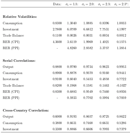
Table 1: Observed and Simulated Moments for IST Shocks Model
Data: σi = 1.5: σi= 2.0: σi = 2.5: σi = 2.5∗:
Relative Volatilities:
Consumption 0.8300 1.3040 1.0885 0.8396 1.0033 Investment 2.7800 6.0709 6.6812 7.7531 4.1997 Trade Balance 0.1100 0.0026 0.0031 0.0034 0.0012 RER (CPI) 4.3600 3.6119 1.9969 1.4021 0.1575 RER (PPI) - 4.8260 2.8582 3.3757 1.3854
Serial Correlations:
Output 0.8800 0.9790 0.9734 0.9623 0.9953 Consumption 0.8900 0.8878 0.9570 0.9160 0.9441 Investment 0.9100 0.6040 0.5453 0.4858 0.7722 Trade Balance 0.8200 0.1968 0.1581 0.1463 -0.1027 RER (CPI) 0.8300 0.6883 0.9549 0.7460 0.8936 RER (PPI) - 0.5933 0.7702 0.5994 0.7059
Cross-Country Correlation:
Output 0.6000 0.9193 0.8657 0.8725 0.8622 Consumption 0.3800 0.6631 0.7468 0.6631 0.5286 Investment 0.3300 0.8866 0.6606 0.7093 0.7379
Notes:The first column refers to data that have been logged and detrended using the HP filter and obtained
from Chari et al.(2002). With the exception of the trade balance, the relative volatility statistics refer to
the ratio of the standard deviation of the variables of interest divided by the standard deviation of GDP. The
standard deviation of the trade balance is simply the standard deviation of the ratio of the trade balance to
GDP.
Figure 1: Home Country’s Response to a 1% IST Shock,σi = 2.5
0 50 100
0 1 2 3
Domestic Intermediate Goods (k 1t)
Years after shock
% Deviation from S−S
0 50 100
−0.8 −0.6 −0.4 −0.2 0
Imported Intermediate Goods (k 2t)
Years after shock
% Deviation from S−S
0 50 100
−1 0 1 2
Total Investment (x t)
Years after shock
% Deviation from S−S
0 50 100
0 0.2 0.4
Total Capital Stock (kt+1)
Years after shock
% Deviation from S−S −0.20 50 100
0 0.2
Domestic Consumption Goods (c1t)
Years after shock
% Deviation from S−S −0.50 50 100
0 0.5
Imported Consumption Goods (c2t)
Years after shock
% Deviation from S−S
0 50 100
−0.1 −0.05 0 0.05 0.1
Total Domestic Consumption (c t)
Years after shock
% Deviation from S−S
0 50 100
−0.05 0 0.05 0.1 0.15
Output of Distribution Services (d t)
Years after shock
% Deviation from S−S
0 50 100
0 0.05 0.1 0.15 0.2
Output of Consumption Goods (y t)
Years after shock
Figure 2: Foreign Country’s Response to a 1% IST Shock,σi = 2.5
0 50 100
−0.6 −0.4 −0.2 0 0.2
Domestic Intermediate Goods (k 2t *)
Years after shock
% Deviation from S−S
0 50 100
0 1 2 3
Imported Intermediate Goods (k 1t *)
Years after shock
% Deviation from S−S
0 50 100
−0.2 0 0.2 0.4 0.6
Total Investment (x t *)
Years after shock
% Deviation from S−S
0 50 100
0 0.1 0.2
Total Capital Stock (k t+1 *
)
Years after shock
% Deviation from S−S −0.20 50 100
0 0.2
Domestic Consumption Goods (c 2t *
)
Years after shock
% Deviation from S−S 00 50 100
0.5 1
Imported Consumption Goods (c 1t *
)
Years after shock
% Deviation from S−S
0 50 100
−0.2 0 0.2
Total Domestic Consumption (c t *)
Years after shock
% Deviation from S−S −0.20 50 100
0 0.2
Output of Distribution Services (d t *)
Years after shock
% Deviation from S−S 00 50 100
0.02 0.04 0.06
Output of Consumption Goods (y t *)
Years after shock
Figure 3: Response of Prices to a 1% IST Shock,σi= 2.5
0 50 100
−0.3 −0.2 −0.1 0 0.1
Foreign Asset Holding (a t+1)
Years after shock
% Deviation from S−S
0 50 100
0 0.05 0.1 0.15 0.2
CPI Real Exchange Rate (rer t c)
Years after shock
% Deviation from S−S
0 50 100
0 0.2 0.4 0.6 0.8
PPI Real Exchange Rate (rer t k)
Years after shock
% Deviation from S−S
0 50 100
−1 −0.5 0 0.5
World Interest Rate (r t)
Years after shock
% Deviation from S−S −0.50 50 100
0 0.5
Domestic Trade Balance (tb t)
Years after shock
% Deviation from S−S 00 50 100
0.01 0.02 0.03
Home Consumer Price Index (p t c )
Years after shock
% Deviation from S−S
0 50 100
0 0.1 0.2
Foreign Consumer Price Index (p t c,*)
Years after shock
% Deviation from S−S −10 50 100
−0.5 0 0.5
Home Producer Price Index (p t k)
Years after shock
% Deviation from S−S −0.10 50 100
0 0.1
Foreign Producer Price Index (p t k,*)
Years after shock
Table 2: Observed and Simulated Moments for TFP Shocks Model Data: σi = 1.5: σi = 2.0: σi= 2.5:
Relative Volatilities:
Consumption 0.8300 0.5262 0.6658 0.9148 Investment 2.7800 0.9391 1.0847 1.5921 Trade Balance 0.1100 0.0024 0.0027 0.0019 RER (CPI) 4.3600 0.8826 0.4946 1.5150 RER (PPI) - 0.7333 0.4140 1.2482
Serial Correlations:
Output 0.8800 0.9700 0.9736 0.9812 Consumption 0.8900 0.9905 0.9945 0.9919 Investment 0.9100 0.9212 0.9696 0.9314 Trade Balance 0.8200 0.6183 0.5072 0.8739 RER (CPI) 0.8300 0.9940 0.9732 0.9709 RER (PPI) - 0.9940 0.9732 0.9709
Cross-Country Correlation:
Output 0.6000 0.3024 0.3199 -0.0161 Consumption 0.3800 -0.1068 0.1131 -0.4974 Investment 0.3300 0.4057 0.4372 -0.3174
Notes:The first column refers to data that have been logged and detrended using the HP filter and obtained
fromChari et al. (2002). With the exception of the trade balance, the relative volatility statistics refer to
the ratio of the standard deviation of the variables of interest divided by the standard deviation of GDP. The
standard deviation of the trade balance is simply the standard deviation of the ratio of the trade balance to
Figure 4: Home Country’s Response to a 1% IST Shoc,σi = 2.5
0 50 100
0 0.5 1 1.5 2
Domestic Intermediate Goods (k 1t)
Years after shock
% Deviation from S−S
0 50 100
0 5 10
Imported Intermediate Goods (k 2t)
Years after shock
% Deviation from S−S
0 50 100
0 1 2 3 4
Total Investment (x t)
Years after shock
% Deviation from S−S
0 50 100
0 0.5 1 1.5
Total Capital Stock (kt+1)
Years after shock
% Deviation from S−S −0.50 50 100
0 0.5 1
Domestic Consumption Goods (c1t)
Years after shock
% Deviation from S−S 00 50 100
5 10
Imported Consumption Goods (c2t)
Years after shock
% Deviation from S−S
0 50 100
0 0.5 1
Total Domestic Consumption (c t)
Years after shock
% Deviation from S−S
0 50 100
−0.5 0 0.5 1
Output of Distribution Services (d t)
Years after shock
% Deviation from S−S
0 50 100
0 0.5 1 1.5
Output of Consumption Goods (y t)
Years after shock
Figure 5: Foreign Country’s Response to a 1% TFP Shock,σi= 2.5
0 50 100
0 0.5 1 1.5
Domestic Intermediate Goods (k 2t *)
Years after shock
% Deviation from S−S
0 50 100
−6 −4 −2 0
Imported Intermediate Goods (k 1t *)
Years after shock
% Deviation from S−S
0 50 100
−0.8 −0.6 −0.4 −0.2 0
Total Investment (x t *)
Years after shock
% Deviation from S−S
0 50 100
−0.4 −0.2 0
Total Capital Stock (k t+1 *
)
Years after shock
% Deviation from S−S −10 50 100
0 1 2
Domestic Consumption Goods (c 2t *
)
Years after shock
% Deviation from S−S −60 50 100
−4 −2 0
Imported Consumption Goods (c 1t *
)
Years after shock
% Deviation from S−S
0 50 100
−0.5 0 0.5
Total Domestic Consumption (c t *)
Years after shock
% Deviation from S−S −10 50 100
0 1 2
Output of Distribution Services (d t *)
Years after shock
% Deviation from S−S −0.20 50 100
−0.1 0
Output of Consumption Goods (y t *)
Years after shock
Figure 6: Foreign Country’s Response to a 1% TFP Shock,σi= 2.5
0 50 100
0 0.2 0.4 0.6 0.8
Foreign Asset Holding (a t+1)
Years after shock
% Deviation from S−S
0 50 100
−2 −1.5 −1 −0.5 0
CPI Real Exchange Rate (rer t c)
Years after shock
% Deviation from S−S
0 50 100
−2 −1.5 −1 −0.5 0
PPI Real Exchange Rate (rer t k)
Years after shock
% Deviation from S−S
0 50 100
−2 0 2 4
World Interest Rate (r t)
Years after shock
% Deviation from S−S −0.20 50 100
0 0.2
Domestic Trade Balance (tb t)
Years after shock
% Deviation from S−S −0.40 50 100
−0.2 0
Home Consumer Price Index (p t c )
Years after shock
% Deviation from S−S
0 50 100
−3 −2 −1 0
Foreign Consumer Price Index (p t c,*)
Years after shock
% Deviation from S−S −10 50 100
−0.5 0
Home Producer Price Index (p t k)
Years after shock
% Deviation from S−S −30 50 100
−2 −1 0
Foreign Producer Price Index (p t k,*)
Years after shock
Table 3: Steady-State Parameter Values:
Parameters: Definitions:
Benchmark:
β= 0.96 Constant annual discount factor
r∗t = 0.04 Steady-state annual world interest rate
δ= 0.10 Constant depreciation rate for Capital stock
α= 0.36 Share of capital services in production
σc = 2.5 Elasticity of sub. between domestic and imported consumer goods
σk= 2.5 Elasticity of sub. between domestic and foreign intermediate goods
σd= 2.5 Elasticity of sub. between dist. svcs and foreign consumer goods
ωc = 0.575 Share of domestic consumer goods
ωd= 0.320 Share of distribution services
ωk= 0.635 Share of domestic intermediate goods
φa= 0.36 Foreign asset adjustment costs
φk = 1.6 Capital adjustment costs (IST Shocks Model)
φk = 0.6 Capital adjustment costs (TFP Shocks Model)
Low Elasticity:
σi= 1.5 Elasticity of sub. between goods
ωc = 0.820 Share of domestic consumer goods
ωd= 0.240 Share of distribution services
ωk= 0.800 Share of domestic intermediate goods
Mid-level Elasticity:
σi= 2.0 Elasticity of sub. between goods
ωc = 0.635 Share of domestic consumer goods
ωd= 0.300 Share of distribution services
APPENDIX 1
A
Derivations and Proofs
A.1 The Problem for the Decentralized Domestic Economy
max
{at+1,c1t,c2t,k1t,k2t,kt+1,kct,kdt,lct,ldt,cm1t,yt,dt}
Et
∞
X
t=0
βtlog(ct), 0< β <1 (37)
s.t.
c1t+p2tc2t+pktk1t+p∗ktk2t+tbt ≤ yt−
φa
2
(at+1−¯a)2 (38)
tbt = at+1−(1 +rt)at (39)
lct+ldt ≤ 1 (40)
kct+kdt ≤ kt (41)
kt+1 = xt+ (1−δ)kt−
φk 2
(kt+1−kt)2 (42)
xt =
h
ωk(k1t)ηk+ (1−ωk)(k2t)ηk
i1
ηk (43)
ct =
h
ωc(c1t)ηc+ (1−ωc)(cm1t)ηc
i1 ηc
(44)
cm1t = hωd(d)ηd+ (1−ωd)(c2t)ηd
i1
ηd (45)
yct = ztkαctl (1−α)
ct (46)
dt = ztkαdtl (1−α)
dt (47)
qt+1 = ρqqt+ρq,q∗q∗t +εqt (48)
zt+1 = ρzzt+ρz,z∗zt∗+εzt (49)
A.2 The FOCs
Usingλc
t,λlt,λkt,λxt,λmt andλdt as the multipliers associated withEquation 38,40,41,42,45
and 47 we have the following first order condition with respect toat+1, c1t,c1tm,c2t,dt,kt+1,
k1t,k2t,kct,kdt,lct and ldt:
λcth1 +φa(at+1−¯a)
i
= βEtλct+1(1 +rt+1) (50)
λct = ωc(c1t)ηc−1
h
ωc(c1t)ηc+ (1−ωc)(cm1t)ηc
i−1
(51)
λm
t = (1−ωc)(cm1t)ηc−1
h
ωc(c1t)ηc+ (1−ωc)(cm1t)ηc
i−1
λctp2t = λmt (1−ωd)(c2t)ηd−1
h
ωd(dt)ηd+ (1−ωd)(c2t)ηd
i
1−ηd
ηd (53)
λd
t = λmt ωd(dt)ηd−1
h
ωd(dt)ηd+ (1−ωd)(c2t)ηd
i
1−ηd
ηd (54)
λx
t[1 +φk(kt+1−kt)] = βEt
n
λx
t+1[(1−δ) +φk(kt+2−kt+1)] +λkt+1
o
(55)
λctpkt = λxtωk(k1t)ηk−1
h
ωk(k1t)ηk+ (1−ωk)(k2t)ηk
i
1−ηk
ηk (56)
λc
tp∗kt = λxt(1−ωk)(k2t)ηk−1
h
ωk(k1t)ηk+ (1−ωk)(k2t)ηk
i
1−ηk
ηk (57)
λkt = λctα yt kct
(58)
λk
t = λdtα
dt
kct
(59)
λlt = λct(1−α)yt
lct
(60)
λlt = λdt(1−α)dt
ldt
(61)
A.3 Deterministic Steady State Conditions
Symmetry in the two economies ensures thatp2t =p1t= 1, similarly, given thatqt=qt∗ = 1
andzt=zt∗ = 1 in steady-state, we must also havetbt= 0 andat=at+1= 0. In steady-state
we haveλi
t=λit+1 =λi ∀i, which implies that β(1 +r) = 1.
FromEquation 50,55,56 and 58:
r+δ =α y kc
ωk(k1)ηk−1
h
ωk(k1)ηk+ (1−ωk)(k2)ηk
i
1−ηk
ηk (62)
FromEquation 50,53,54,55,56 and60:
r+δ=α d kd
ωd 1−ωd
c2
d
ηd−1
ωk(k1)ηk−1
h
ωk(k1)ηk + (1−ωk)(k2)ηk
i
1−ηk
ηk
(63) FromEquation 53,54,60 and 61:
d
y
lc
ld
=1−ωd
ωd
d
c2
1−ηd
(64) FromEquation 56and 57:
k1
k2
=h ωk 1−ωk
i1−1 ηk
(65) FromEquation 51, Eq.52 and 53:
c1
cm 1
=h1−ωc
ωc
(1−ωd)
h
ωd
d
c2
ηd
+ (1−ωd)
i
1−ωd
ωd i
1
ηc−1
To complete the deterministic steady-state conditions we have the following constraints:
lc+ld = 1 (67)
kc+kd = k (68)
ωk
k1
k2
ηk
+ (1−ωk) =
δk
k2
ηk
(69)
ωd
d
c2
ηd
+ (1−ωd) =
cm
1
c2
ηd
(70)
d kd
= kd
ld
α−1
(71)
y kc
= kc
lc
α−1
(72)
y = c1+c2+k1+k2 (73)
To fully calibrate the steady-state we have a system of 12 equations and 12 unknown. The unknowns we need to solve for are: y,kc,kd,lc,ld,k,k1,k2,d,c1,c2, andcm1 . We use the factor
price equalization condition in both the labor and capital markets to obtain cd2 = ωd
1−ωd 1−1
ηd
and kd
ld =k=
kc
lc. These two conditions, along with the value of
k1
k2 can then be used to obtain