Full Length Research Article
STRUCTURAL DYNAMICS OF THE MONEY SUPPLY IN BENIN FROM 2001 TO 2012
*
Vincent Jean-Marie Kiki
Statistician-Economist, Lecturer and Head of department, Ecole Nationale d’Economie Appliquée et de
Management/ Université d’Abomey-Calavi, ENEAM/UAC, République du Bénin (UAC)
ARTICLE INFO ABSTRACT
This study found that the main component of the money supply before 2003 was banknotes in circulation. From 2003 to 2012, demand and term deposits are the main components of the money stock. An econometric analysis, through an error correction model, revealed that all the variables, namely, the monetary supply, the monetary base, the credits to the economy, net foreign assets and the interest rate are integrated of the order 1 and the residuals of the order 0. Therefore, there is a co-integrating relationship between them. Monthly data over the period 2001-2012 were used. They came from BCEAO (monthly newsletters, integrated monetary statistics, etc.). The results revealed that all the variables are significant in the short and long run, except the interest rate (0.03% in long run and -0.04% in short run). Thus, as Adjovi (2010) stated, the commercial banks are increasingly brought to ignore signals from the central bank. Even if the central bank cuts interest rates, the primary banks do not decrease their base rate. In WAEMU countries, in general, and in Benin in particular, the transmission of monetary policy to the real sphere, is lacking.
Copyright © 2014 Vincent Jean-Marie Kiki. This is an open access article distributed under the Creative Commons Attribution License, which permits
unrestricted use, distribution, and reproduction in any medium, provided the original work is properly cited.
INTRODUCTION
Money is a consensual payment instrument occurred in the 14th century to the detriment of barter. Therefore, trade ceased to be complex operations of direct disposal of tangible property against another. In Benin and according to statistics released by the CAPOD in 2009, the money stock in circulation increased by 288.88%, and therefore has almost tripled in 2009 compared to 2000 (Adjovi 2009). What is the structural dynamics explaining the growth rate of the money supply? It seems relevant to provide an answer to this research question, for the sake of contributing a little bit, some lighting in terms of monetary policy in Benin. Thus, this article aims to study the evolution of the money supply in relation to the evolution of its essential components and counterparts. In Benin, WAEMU country, the money stock is considered to be composed by: the banknotes and coins in circulation, demand and term deposits. Overall, the counterparts of the money supply are: the credit to the economy, net foreign assets and net government position. These counterparts are indeed likely to impact the money supply through certain forces, whose evolution is relevant to be analyzed.
*Corresponding author: Vincent Jean-Marie Kiki
Statistician-Economist, Lecturer and Head of department, Ecole Nationale d’Economie Appliquée et de Management/ Université d’Abomey-Calavi, ENEAM/UAC, République du Bénin (UAC)
Specifically, this study aims to:
• Describe the evolution of the money stock; • Describe the components of its structure;
• To analyze the effect of its counterparts on the money supply.
The interest of this study lies in the fact that it is likely to open or to confirm the ways of adjustments and improvement of monetary policy in Benin. Its originality lies in the dynamic approach, which assumes a cross look of the evolution of the money supply and its constituents and the forces that represent the effects of the counterparties of the money supply. The study focuses on four key areas including, firstly, the context and objectives of the research. The second axis addresses through a brief literature review issues related to the theoretical framework of the research. The third part presents the methodology, while the fourth and last axis is that of the results and discussion.
Theoretical framework
It declines the main key concepts and theories used in this study.
Conceptual approach
Among the salient concepts in this article, it may be noted fundamentally: the monetary base and the money supply.
ISSN:
2230-9926
International Journal of Development Research
Vol. 4, Issue, 8, pp. 1520-1527, August,2014
International Journal of
DEVELOPMENT RESEARCH
Article History:
Received 20th May, 2014 Received in revised form 18th June, 2014 Accepted 30th July, 2014 Published online 05th August, 2014
Key words:
Money supply, Structural dynamics, Benin
The monetary base
It is composed by bank reserves beside the central bank as well as banknotes and coins in circulation.
The money stock and its structure
The money stock is the amount of money in circulation in an economy at a given time. It includes all the assets held by non-financial economic agents (households, rest of the world, state, enterprises) to finance their consumption or investment. These assets consist of various elements. Thus, one defines a set of "monetary aggregates" that reflect the composition of these assets. There are three monetary aggregates, namely M1, M2 and M3.
The M1 monetary aggregate
This is the monetary availability or the money stock in the strict sense. It includes all the instruments that can be used directly as a means of payment without prior processing and without cost. This is the most liquid money. It includes banknotes in circulation and demand deposits. The demand deposits are bank deposits that are freely available to economic agents at any time without limitation.
M1 =Banknotes in Circulation + Demand deposits
The M2 monetary aggregate
Also called broad money stock or simply money stock, it consists of the M1 aggregate and the quasi-monetary availability. Quasi money includes assets that do not have a perfect degree of liquidity, but whose transformation into a means of payment directly mobilizable requires a short time and generates relatively low cost.
M2 = M1 + Quasi money
With: Quasi money = Small-denomination time deposits and repurchase agreements + Savings deposits and money market deposit accounts + Money market mutual fund shares (non-institutional). M2 is basically used in the WAEMU (West African Economic and Monetary Union).
The M3 monetary aggregate
Also called total liquidity in the economy, it is the broadest monetary aggregate. It is composed of the M2 money supply and deposits in saving accounts of Treasury and in other saving accounts. These deposits include mainly the following:
• Treasury bills: these are securities issued by the State to households, companies and banks to meet expenses not covered by budgetary revenues.
• Savings accounts with the saving banks: it is a type of deposit account paid benefiting from financial and tax benefits and whose interests are calculated per fortnight. • Housing savings accounts with the saving banks: these are
unavailable deposits for a minimum period (4 years) and requiring a minimum deposit, followed by annual deposit greater than or equal to a specified amount.
M3 = M2 + Treasury bills+ Savings accounts with the saving banks + Housing savings accounts with the saving banks.
The structure of the money stock and some theoretical approaches
Regarding Benin economy, the concept of the money stock is represented by M2 described above.
The structure of the money stock
As an aggregate M2, it appears that the money stock, as seen in Benin, is structured as follows: there are notes and coins in circulation, demand deposits and term deposits.
• Notes and coins in circulation: there are notes and coins in circulation in the economy, except for banknotes and coins in circulation stored by banks.
• Demand deposits: There are the total deposits by non-financial economic agents, with non-financial institutions, which they may dispose freely at any time.
• Term deposits: they are a form of deposits, but whose duration is fixed at the request. These deposits create a shot if you ask repossess these assets before the set time.
The study of the evolution of these structural elements of the money supply is made later by a simple descriptive statistical analysis. These components have as counterparties, credits to the economy, the net foreign assets and claims on the state.
Counterparts of the money stock
The counterparts of the money stock include claims that correspond to the various monetary aggregates that are defined above. They allow knowing which economic agents have contributed to the formation of the money stock. It is basically: net foreign assets, credits to the economy, and credits to the state.
Net foreign assets
They measure the impact of the current account of the balance of payments and balance of capital movements in the short and long term of non-financial agents on the monetary assets of residents.
Credits to the economy
They correspond to the main counterparts of the money stock. They represent all loans to companies for their cash needs or to finance their investments, and all loans to households.
Claims on the Treasury
They measure the counterpart on the state, which makes appeal to the banking system for short-term refinancing. Some of these variables, including the first two will be used later in an econometric model, explaining their impact on the evolution of the money stock, only endogenous variable of the study. Regarding to the monetary base, it will be used in the model as an exogenous variable.
The money supply
A simple approach states that money creation by the central bank may be directed by the monetary authorities, to pursue policies in order to achieve a number of objectives such as price stability, full employment and growth. An illustration is a statistical study carried out by Walters (1966) in UK. This study showed that from 1955 to 1962, the British government varied the money supply as an inverse function of price movements and the deficit of the trade balance recorded in previous quarters. This action is in fact, the policy of "stop and go" practiced in UK after the Second World War. It is a policy of reducing the money supply as soon as emerged a situation of expansion of demand, resulting in a risk of inflation, followed by a recovery policy as soon as the previous braking sparked an early recession. Thus, the result revealed that a 1% increase in prices leads the authorities to reduce the money supply by 0.9%, which means 0.65% in the quarter following the price change, and 0.32% thereafter. In Burundi, Ntandikiye (2000) examined the influence of economic variables on the money supply. Having reviewed the confrontation of ideas of many authors and theories developed around the money supply, he argued that monetary phenomenon is very complex and that its inclusion can work in different ways. Based on an Error Correction Model, he concluded that the monetary base is not really exogenous is Burundi. Ouedraogo (2004) investigated the determinants of the money supply in the WAEMU countries, using an Error Correction Model (ECM) explaining the variations of the quantity of money. He found that in the short term, monetary base, bank deposits and public cash coefficient influence the money supply. In the long term, money supply is driven by deposits.
Methodological Framework
It has two components: a descriptive analysis of money supply and an econometric approach.
Descriptive analysis
The descriptive analysis was to describe the evolution of the money supply and its components in Benin from 2001 to 2012. The strategy adopted is a simple graphical description in Excel.
The econometric model
The econometric analysis captures the evolution of the money supply implicitly related to the action of the forces exerted by its counterparts.
Variables of the econometric model
The endogenous variable is the money supply (MM). There are four exogenous variables: the monetary base (BM), the credits to the economy (CRE), net foreign assets (AEN) and the interest rate (TXINT). Credits to the economy and net foreign assets are the main counterparts of the money stock. Their inclusion in the model is to capture the bulk of the forces exerted by the counterparts on the money stock through its structure. Indeed, a Principal Component Analysis (PCA) revealed that the effect of the third counterpart (claims on the state) is negligible. Variables that attract attention are: the monetary base, the credits to the economy, net foreign assets, and the interest rate. Indeed the analysis of the correlation
matrix, with SPAD, showed that these variables influenced mainly the money supply. Thus, among the three counterparts, PCA highlights the predominance of credits to the economy and net foreign assets at the expense of claims on the state.
Model specification
The model is:
MMSA= c + 1BMSA + 2CRESA + 3AENSA + 4TXINT (1)
or
LMM= c + 1LBM + 2LCRE + 3LAEN + 4LTX (2)
where L is the logarithm.
Data
This study resorted to monthly data over a period of 12 years, thus 144 observations. The data are mainly from the integrated monetary statistics (SMI), monthly bulletins of the Banque Centrale des Etats de l’Afrique de l’Ouest (BCEAO) and databases from the web site of the Central Bank. They are relative to the money supply, the monetary base, the credits to the economy, net foreign assets, and the interest rate.
Data Processing
The analyses were carried out with EVIEWS. Model variables were seasonally adjusted. Unit root tests and co-integration were performed on the variables. The finding revealed that the variables are integrated of the same order, which gives the possibility of implementing an ECM.
Analysis of the seasonality of the series
Analysis of the seasonality
A prerequisite for the study of stationarity of time series is the analysis of seasonality. Indeed, it is necessary to correct the sub-annual series from seasonal variations before analyzing them. The seasonal adjustment is done by the means of Moving Average Method (MAM) with Eviews 5.0. In the literature, there are generally three (03) types of models to describe seasonality:
• The additive model: Xt = Tt + St + ɛt
• The multiplicative model: Xt = Tt * St * ɛt
• The mixed model: Xt = Tt * St + ɛt
Buys-Ballot test
Buys-Ballot test is based on analytical methods, taking into account the averages, Xt, and standard deviation, σt, for each
period (year). For these pairs of observations (͞Xt, σt), we
estimate by OLS the parameters a and b of the equation σt=a+b*͞Xt+ɛt. If the coefficient is not significantly different
from 0, we accept the hypothesis of an additive scheme; otherwise, it is a multiplicative scheme.
Unit root tests
are stationary or not. By definition, a time series is stationary if its mean and variance are constant over time, and the value of covariance between two time periods depends only on the distance or gap between the two periods and not on the time at which the covariance is calculated. More specifically, it is to carry out unit root test on these series. For this purpose, Augmented Dickey-Fuller test is performed. This test helps to detect the existence of a trend and also to determine the best way to make a series stationary. The null hypothesis, H0,
(presence of unit root) is tested against the alternative hypothesis, H1, (no unit root) by referring to the values shown
in DF table. The decision rule is as follows:
• if the calculated value of the t-statistic associated with λ is less than the tabulated critical value, we reject the null hypothesis of unit root: the time series is stationary; • if the calculated value of the t-statistic associated with λ
is greater than the tabulated critical value, we do not reject the null hypothesis of non-stationarity.
Co-integration and error correction model
Co-integration
The concept of co-integration provides the theoretical framework for studying situations of balance and imbalance, prevailing respectively in the long and short run. If the variables are co-integrated, they admit an error correction specification that transforms the initial regression problem on non-stationary variables. Co-integration allows identifying the true relationship between two variables, by identifying the existence of a co-integrating vector and eliminating its effect, if any. Two series Yt and Xt are co-integrated, if the following
two conditions are satisfied:
• they are assigned a stochastic trend of the same order of integration, d, that is to say: Yt --> I(d) and Xt --> I(d)
• a linear combination of these series can be reduced to a series of lower order of integration: α1 Yt + α2 Xt -->I
(d-b) with d≥b>0. [α1; α2] is called co-integration vector.
The co-integration tests that can be used are Johansen test and Engel and Granger test.
Engel-Granger co-integration test
This test is done in two steps:
• Estimate the long-run model based on integrated variables in the same order by Ordinary Least Squares (OLS).
• Recover the residuals of the long-run relationship and to test their stationarity. When the residuals are stationary, the co-integration relationship is accepted.
Johansen co-integration test
The co-integration test developed by Johansen in 1988 is based on the rank of the coefficient matrix of the vector of variables of interest (Y) to their greatest lag in the model. The Johansen test includes a test based on the trace and another on the maximum eigenvalues. This study uses the test based on the trace, assuming no trend in the co-integrating relationship and the presence of a constant in the ECM.
Error Correction Model (ECM)
When the series are non-stationary and co-integrated, one should estimate their relationships through an ECM. Engel and Granger (1987) showed that all co-integrated series can be represented by an ECM. The method proceeds in two steps, according to the following procedure:
Step 1:
The long-run model is estimated between co-integrated variables in the model and the residuals are generated. The residuals are test for stationarity.
Yt = β + λXt + εt
Step 2:
The residuals are lagged and introduced into the short-run model:
Yt = α1Xt + α2εt-1 + εt
A necessary but not sufficient condition to validate the estimated model is to obtain a coefficient (α2), called error
correction coefficient, which must be negative and significantly different from zero. The ECM is a model that incorporates both the short-term developments around a long-run equilibrium. After studying the nature of the variables, the model is estimated. The estimation is run using EVIEWS. The goal is to quantify the influence of different variables on the evolution of the money stock. After estimating the model, it is worth checking its validity. This is based on six main tests. These include the Breusch-Godfrey autocorrelation test, White heteroskedasticity test, normality test, Fisher test of overall significance, Student test on individual quality of coefficients and CUSUM stability test.
Results and Discussion
On the evolution of the money stock and its counterparts
Evolution of the money stock
Source: Author, with Excel
Figure 1. Evolution of the money stock from 2001 à 2012
[image:5.595.40.556.316.501.2]Source: Author, with Excel
Figure 2. Structure of the money stock
Source: Author, with Excel
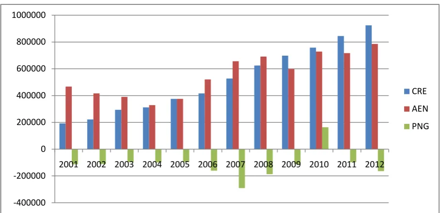
Figure 3. Compared evolution of the counterparts of the money stock
0 200000 400000 600000 800000 1000000 1200000 1400000 1600000 Ja n -0 1 Se p -0 1 M ay -0 2 Ja n -0 3 Se p -0 3 M ay -0 4 Ja n -0 5 Se p -0 5 M ay -0 6 Ja n -0 7 Se p -0 7 M ay -0 8 Ja n -0 9 Se p -0 9 M ay -1 0 Ja n -1 1 Se p -1 1 M ay -1 2
MM
MM 0% 10% 20% 30% 40% 50% 60% 70% 80% 90% 100% Ja n -0 1 Ju l-0 1 Ja n -0 2 Ju l-0 2 Ja n -0 3 Ju l-0 3 Ja n -0 4 Ju l-0 4 Ja n -0 5 Ju l-0 5 Ja n -0 6 Ju l-0 6 Ja n -0 7 Ju l-0 7 Ja n -0 8 Ju l-0 8 Ja n -0 9 Ju l-0 9 Ja n -1 0 Ju l-1 0 Ja n -1 1 Ju l-1 1 Ja n -1 2 Ju l-1 2 dt dv CF -400000 -200000 0 200000 400000 600000 800000 10000002001 2002 2003 2004 2005 2006 2007 2008 2009 2010 2011 2012
CRE
AEN
[image:5.595.69.524.537.757.2]evolution of the socio-economic situation in the country. In 2005, the economic situation was characterized by a growth rate of 3.5% against 3.4% in 2004, due to the dynamics of the secondary and tertiary sectors. The tertiary sector is driven by the favorable impact of the resumption of trade with Nigeria. This economic growth has, however, not been continue in 2009 due to the effects of the international financial crisis, and the measures taken by Nigeria to deal with the food crisis. In 2009, the growth rate was estimated at 2.7%. Benin's government took measures to lighten the living conditions of populations, and the money supply has thus not been greatly affected by the various crises.
Evolution of the structure of the money stock
Figure 2 (Appendices) shows the structure of the money stock, shared between the banknotes in circulation, demand deposits and term deposits. Between 2001 and 2006, banknotes in circulation have emerged as a major component of the money stock. It marks sometimes a slight decrease to the benefit of demand deposits that became more important since 2009. They represent, over the period 2007-2009, nearly 40% of the money stock, evolving almost in equal proportion with term deposits. Since 2010, term deposits became the most important components of the money stock (40% of money stock), letting evolved in equal proportion banknotes in circulation and demand deposits. On average, the money stock evolved following the evolution of deposits over the recent years. It should, nevertheless, be noted that the choice of Beninese economic agents reflect the actual economic situation. They choose to save more, in order to defer consumption in a future they hope better.
Evolution of the counterparts of the money stock
Since the 2000s, claims on the state decreased - net government position - (Figure 3 -Appendices-). The debt position of the government in 2007 reached 35% of the money stock. Despite fiscal consolidation, resulting in rationalization of expenditure and debt collection, the state continued to be in a situation of chronic deficit. The net foreign assets seemed to evolve like the money stock. Both of the two series move synchronously. The net foreign assets have imposed their changes to the money stock until 2008. This rhythmic evolution broke since 2008. The international economic situation has not been without effect on the level of net foreign assets available in the Beninese economy. Despite a change sometimes marked by ruptures, it is note an increasing evolution of the money supply over this period, with concordance with its counterparts. Also credits to the economy were proliferating. They have been trending upward since 2001.
Results of estimation
[image:6.595.311.556.76.126.2]The unit root tests reveal that all the variables are non stationary at level, and are stationary at the first difference. Thus, they are integrated of order one. Both of the Engle-Granger and Johansen co-integration tests indicate that the series are co-integrated. Therefore, it is appropriate to estimate the relationship between variables through an ECM by Engle-Granger two-step method.
Table 1. Synthesis of Buys-Ballot test
Variable Modèle décrivant la saisonnalité Variable désaisonnalisée
MM Additif MMSA
BM Additif BMSA
AEN Additif AENSA
CRE Multiplicatif CRESA
Source : Author, with Excel
Table 3. Unit root test on long-run residuals
Variables ADF test
statistic t-statistic Prob. Modèle
Ordre d’intégration
Residuals -14,22153 -1,943090 0,0000 1 0
[image:6.595.306.561.169.236.2]Source: Author with Eviews
Table 4. Results of trace test on the logarithmic values
Test (Trace) Hypothesiz
ed No. of
CE(s)
Eigen value Trace
Statistic
0.05 Critical
Value
Prob**
None * 0.277488757 83.58478278 60.06140647 0.000163690
At most 1 0.129797971 38.40668324 40.17493178 0.074493005
At most 2 0.088690159 19.08153022 24.27595860 0.196614893
At most 3 0.034277991 6.172276469 12.32089895 0.415304914
At most 4 0.009480379 1.324058985 4.129906228 0.292096959
[image:6.595.307.559.351.443.2]Source: Author, with Eviews
Table 5. Results of the test of maximum eigen value
Test (Maximum Eigen value) Hypothesize
No. of CE(s) Eigen value
Max-Eigen Statistic
0.05
Critical Value Prob**
None * 0.27748875 45.17809954 30.43961085 0.000388788
At most 1 0.12979797 19.32515301 24.15920873 0.197578754
At most 2 0.08869015 12.90925375 17.79729850 0.233709058
At most 3 0.03427799 4.848217483 11.22479930 0.498926543
At most 4 0.00948037 1.324058985 4.129906228 0.292096959
[image:6.595.306.561.484.559.2]Source : Author, with Eviews
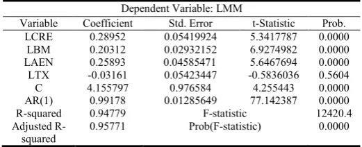
Table 6. Results of long-run model
Dependent Variable: LMM
Variable Coefficient Std. Error t-Statistic Prob. LCRE 0.28952 0.05419924 5.3417787 0.0000
LBM 0.20312 0.02932152 6.9274982 0.0000 LAEN 0.25893 0.04585471 5.6467694 0.0000 LTX -0.03161 0.05423447 -0.5836036 0.5604 C 4.155797 0.976584 4.255443 0.0000 AR(1) 0.99178 0.01285649 77.142387 0.0000 R-squared 0.94779 F-statistic 12420.4 Adjusted
R-squared
0.95771 Prob(F-statistic) 0.0000
Source : Author, with Eviews
Estimation and validation of the long-run model
Estimated long-run model (Table 6 -Appendices-)
The estimated long-run model is:
Table 2. Synthesis of unit root test
Variables ADF test
statistic t-statistic Prob. Modèle
Ordre d’intégration
LMM -10,30059 -2,881978 0.0000 2 1
LBM -2,996115 -1,943304 0,0030 1 1
LCRE -6,375179 -2,882433 0,0000 2 1
LAEN -10,21497 -1,943107 0,0000 1 1
LTX -10,25107 -1,943090 0,0000 1 1
[image:6.595.302.563.599.705.2] Validation of long-run model
[image:7.595.52.271.382.455.2]The tabulated value of the Student statistic at 5%, and at degree of freedom of 144-3 = 141 (with 144: the number of observations and 5: the number of parameters) is equal to 1.96. This value is less than the t-statistics for all variables, except the interest rate. Therefore, the quality of individual estimators is good for all variables, except for the interest rate. R2 = 0.947799, which is very close to unity, showing that the model is well specified. This is confirmed by the Fischer test whose probability associated to its calculated statistic (Table 7) is less than the 5% threshold. Hence, the regression is overall significant. J-B = 5.24, and thus, the residuals are normal (Indeed, J-B <5.99). The probability is equal to 0.072530 (see Appendix 8.1.1). The application of Breusch-Godfrey test at order 2 yields a probability equal to 0.051952> 5% (see Appendix 8.1.2), so we conclude that there is no autocorrelation of errors. The White heteroskedasticity test shows that the errors are homoskedastic. Indeed, the probability is 0.653706> 5% (see Appendix 8.1.3).
Table 7. Synthesis of the tests on the individual quality of the estimators and the overall quality of the long-run model
C LBM LCRE LAEN LTX
Student
statistics 4,25 6,92 5,34 5,64 -0,58 R2
0,947799 Fischer
Statistic 12420,46
Source : Author, with Eviews.
Estimation and validation of the short-run model
Estimation of short-run model (Table 8 -Appendices-)
The estimated model is:
With ~>WN (White Noise). Variables D(LMM), D(LCRE) D(LBM), D(AENSA) and D(TXINT) are the first difference of LMM, LCRE, LBM, LAEN, LTX.
Validation of the short-run model
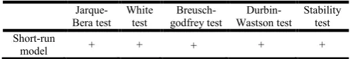
The R-squared is 0.76; the explanatory variables explain well the endogenous variable. Thus, changes in the money stock are explained in both the short and long run by credits and net foreign assets in priority, and also by the monetary base. In the short-run model, J-B = 1.223436, and the residuals are normal (Indeed, J-B <5.99). The probability is equal to 0.542418 (see Appendix 8.2.1). The Breusch-Godfrey test at order 2 yields a probability equal to 0.259680> 5% (see Appendix 8.2.2), so we conclude that there is no autocorrelation of errors. The White heteroskedasticity test shows that the errors are
homoskedastic. Indeed, the probability is 0.062215> 5% (see Appendix). The Cusum stability test shows that the curve does not cross the corridor, and then the model is structurally stable. It can be used for forecasting purposes (See Appendix 8.2.3). The error correction coefficient is significant (probability=0.0002) and negative (value of - 0.212196), and then the ECM is validated.
Economic analysis of the results
The results show that the variables namely, the monetary base, net foreign assets, credits to the economy and interest rate influence the money supply. Indeed, the coefficients of the first three variables are positive in both long and short run, and the last variable has a negative coefficient in the short run. The model is overall significant in both long and short run, that is to say the independent variables have an influence on the dependent variable.
The monetary base
Student test shows that the monetary base has positive and significant impact on the money supply (see Table 7, Table 8 -Appendices-). Thus, in the long run, a 1% increase in the monetary base implies an increase of 0.203% of the money supply. This impact remains the same regarding the short run. Indeed, the results show that a 1% increase in the monetary base leads to an increase of 0.204% in the money stock in short run. These results highlight the fact that the monetary base influences the money supply in the long short run, but also the exogeneity of the money supply in Benin.
Table 8. Results of short-run model
Dependent Variable: D(LMM)
Variable Coefficient Std. Error t-Statistic Prob. D(LCRE) 0.28045 0.053329 5.258880 0.0000
D(LBM) 0.20442 0.029200 7.000831 0.0000 D(LAEN) 0.26437 0.045338 5.831257 0.0000 D(LTX) -0.04392 0.053464 -0.821527 0.4128 RESID01(-1) -0.21219 0.085766 -2.474130 0.0146 D2008 0.00868 0.005904 1.470758 0.1437 C 0.00138 0.001795 0.773992 0.4403 R-squared 0.76886 F-statistic 74.8450 Adjusted
R-squared
0.75859 Prob(F-statistic) 0.00000
[image:7.595.301.564.440.556.2]Source: Author, with Eviews
Table 9. Synthesis of validity tests on the short-run model
Jarque-Bera test
White test
Breusch-godfrey test
Durbin-Wastson test
Stability test Short-run
model + + + + +
Source : Author, with Excel
Net foreign assets
[image:7.595.305.561.594.637.2]Credits to the economy
The effects of changes in the credits to the economy on the money supply are observed over the long and short run. In the short run, the impact on the evolution of the money supply is less important compared to the long run. Indeed, a 1% increases of credits to the economy impulse in the long run an increase of 0.29% and a 0.28% increase in the money supply in the short run. This variable appears as a key variable in controlling the money supply, since its impact is the most important on the evolution of the quantity of money in circulation.
The interest rate
The interest rate has a positive effect on the money supply in the long run, but the effect is not significant. In the short run, the impact of this variable is insignificant. It is observed that, in Benin, the interest rate cannot be used wisely as a monetary-policy variable, because its mechanisms are not transmitted earlier. Adjovi (2010) stated that: "The current configuration of the banking system leads the commercial banks to not take sufficient account of the signals transmitted by the Central Bank. Indeed, even if the Central Bank decreases the interest rate, the primary banks do not decrease their base rate. Thus, the transmission of monetary policy to the real sector in the WAEMU countries in general, and Benin in particular, is not obvious, and sometimes non-existent."
Interpretation of the error correction coefficient
It is noted that the coefficient associated with the lagged residuals is significantly negative (-0.212196) at 5% (the absolute value of its t-Statistic is greater than 1.96). So there is an error correction mechanism. In the long run, imbalances between bank deposits, credits to the economy, net foreign assets and the interest rate are offset so that the series have similar trends. 21.21% of imbalances between the desired level and the actual level of the money supply are adjusted in the current period. Thus, the shocks on the overall level of growth will fade after 4 months, 21 days 9 hours (1/0. 212196 months). In other words, it is the time of adjustment, that is to say the time necessary to ensure its return to equilibrium.
Conclusion
The Structural dynamics of the money supply in Benin for the period 2001-2012 is justified both, by the joint description of the evolution of the money supply and its components, as well as those of its counterparts, whose evolutionary effects can be seen as a series force infusing some dynamics to the money in circulation in Benin from 2001 to 2012. It should be emphasized on the fact that the money supply and its counterparts undergo upward trend over the period of study,
while being remarkably unstable, in the image of the international economic situation. The analysis of the ECM allowed highlighting the influence of four variables on the dynamics of the money supply. The study revealed that the money supply responds positively to changes in the monetary base, credits to the economy and net foreign assets. Regarding the interest rate, it seems to be ineffective as a variable of monetary policy in Benin. The interest of this study lies in the fact that, in terms of monetary policy in Benin, credits to the economy and net foreign assets appear as the variables that the government can effectively control, in one way or another in regard to the expected impacts and outcomes of monetary policy.
Competing Interests: No competing interests exist
REFERENCES
BCEAO. 2007. Lien entre la masse monétaire et l'inflation dans les pays de L'UEMOA, Document d’Etude et de Recherche N° DER/07/02 Mai 2007.
Agence Monetaire De L’afrique De L’ouest (AMAO). 2009. Croissance de la masse monétaire et convergence macroéconomique au sein de la CEDEAO.
BCEAO. 2007. Bulletin de Statistiques Monétaires et Financières, Décembre 2007.
BCEAO. 2008. Bulletin de Statistiques Monétaires et Financières, Juin 2008.
Claassen, E. 1981. Macroéconomie: bases de la théorie monétaire, Editions BORDAS, Paris
Doucoure, F. B. 2005. Méthodes économétriques et Programmes, Editions CREA, Sénégal.
Adjovi, E. G. S. 2010. Politiques Macroeconomiques Au Benin : progrès, limites et perspectives, Document de Travail n° 010/2010 du CAPOD (Cabinet d’Analyse de Politique de Développement.
Mankiw, G. N. 2003. Macroéconomie, Editions Nouveaux Horizons, 3e édition, Bruxelles.
Ntandikiye, T. 2000. Les déterminants de l’offre de monnaie et l’exogénéité de la base monétaire exogène au Burundi : théorie et vérifications empiriques.
Ouedraoguo, A. 2004. Déterminants de l’offre de monnaie dans l’UMOA, Editions ENSEA, Abidjan.
Castex, P. 2000. Le miracle de la création monétaire, Alternatives Economiques, Hors-série : La monnaie, n°45, 2000, pp. 32-33.
UEMOA. 2011. Rapport sur la politique monétaire dans l'UEMOA, Décembre 2011.
UEMOA. 2002. Rapport sur la politique monétaire dans l'UEMOA, Mars 2013.
Walters, A. 1966. Monetary multipliers in the United Kingdom, Oxford Economic Papers.