Munich Personal RePEc Archive
The bipolar Choquet integral
representation
Greco, Salvatore and Rindone, Fabio
Faculty of Economics, University of Catania
August 2011
Online at
https://mpra.ub.uni-muenchen.de/38957/
The Bipolar Choquet Integral Representation
Salvatore Greco
∗, Fabio Rindone
†Faculty of Economics, University of Catania,
Corso Italia, 55, 95129 Catania, Italy
Abstract
Cumulative Prospect Theory of Tversky and Kahneman (1992) is the modern version of Prospect Theory (Kahneman and Tversky (1979)) and is nowadays considered a valid alternative to the classical Expected Util-ity Theory. Cumulative Prospect theory implies Gain-Loss Separability, i.e. the separate evaluation of losses and gains within a mixed gamble. Recently, some authors have questioned this assumption of the theory, proposing new paradoxes where the Gain-Loss Separability is violated. We present a generalization of Cumulative Prospect Theory which does not implyGain-Loss Separability and is able to explain the cited para-doxes. On the other hand, the new model, which we call the bipolar Cumulative Prospect Theory, genuinely generalizes the original Prospect
Theory of Kahneman and Tversky (1979), preserving the main features of the theory. We present also a characterization of thebipolar Choquet Integral with respect to abi-capacity in a discrete setting.
Key words: Cumulative Prospect Theory, Gains-Loss Separability, bi-Weighting Function, Bipolar Choquet Integral.
JEL ClassificationD81·C60
∗salgreco@unict.it, Tel. +39 095.7537733 - Fax +39 095-7537510
1
Introduction
Cumulative Prospect Theory (CPT) of Tversky and Kahneman (1992) is the modern version of Prospect Theory (PT) (Kahneman and Tversky (1979)) and is
nowadays considered a valid alternative to the classical Expected Utility Theory (EUT) of Von Neumann and Morgenstern (1944). CPT has generalized EUT,
preserving the descriptive power of the original PT and capturing the fundamen-tal idea of Rank Dependent Utility (RDU) of Quiggin (1982) and of Choquet
Expected Utility (CEU) of Schmeidler (1986, 1989) and Gilboa (1987). In re-cent years CPT has obtained increasing space in applications in several fields: in
business, finance, law, medicine, and political science (e.g.,Benartzi and Thaler (1995); Barberiset al.(2001); Camerer (2000); Jollset al.(1998); McNeilet al.
(1982); Quattrone and Tversky (1988)). Despite the increasing interest in CPT - in the theory and in the practice - some critiques have been recently
pro-posed: Levy and Levy (2002); Blavatskyy (2005); Birnbaum (2005); Baltussen
et al.(2006); Birnbaum and Bahra (2007); Wu and Markle (2008); Schadeet al.
(2010). In our opinion, the most relevant of these critique concerns the
Gain-Loss Separability (GLS), i.e. the separate evaluation of losses and gains. More precisely, let P = (x1, p1;. . .;xn, pn) be a prospect giving the outcome xi ∈R
with probabilitypi, i=1, . . . , nand letP+(P−)be the prospect obtained fromP
by substituting all the losses (gains) with zero. GLS means that the evaluation of P is obtained as sum of the value ofP+and P− : V(P) =V(P+) +V(P−).
Wu and Markle (2008) refer to the following experiment: 81 participants gave
their preferences as it is shown below (readH ≻ L“the prospectHis preferred to the prospect L”)
H = ⎛ ⎜⎜ ⎜⎜ ⎜ ⎝
0.50chance at$4,200
0.50chance at$−3,000
⎞ ⎟⎟ ⎟⎟ ⎟ ⎠ ≻ ⎛ ⎜⎜ ⎜⎜ ⎜ ⎝
0.75chance at$3,000
0.25chance at $−4,500
⎞ ⎟⎟ ⎟⎟ ⎟ ⎠ = L
[52%] [48%]
H+=
⎛ ⎜⎜ ⎜⎜ ⎜ ⎝
0.50chance at$4,200
0.50chance at$0
⎞ ⎟⎟ ⎟⎟ ⎟ ⎠ ≺ ⎛ ⎜⎜ ⎜⎜ ⎜ ⎝
0.75chance at$3,000
0.25chance at$0
⎞ ⎟⎟ ⎟⎟ ⎟ ⎠
= L+
H−=
⎛ ⎜⎜ ⎜⎜ ⎜ ⎝
0.50chance at$0
0.50chance at$−3,000
⎞ ⎟⎟ ⎟⎟ ⎟ ⎠
≺
⎛ ⎜⎜ ⎜⎜ ⎜ ⎝
0.75chance at$0
0.25chance at $−4,500
⎞ ⎟⎟ ⎟⎟ ⎟ ⎠
= L−
[37%] [63%]
As can be seen, the majority of participants preferred Hto L, but, when the two prospects were split in their respective positive and negative parts, a
rel-evant majority prefers L+ to H+ and L− to H−. Thus, GLS is violated and CPT cannot explain such a pattern of choice. In the sequel we will refer to this
experiment as the “Wu-Markle paradox”.
In the CPT model the GLS implies the separation of the domain of the gains
from that of the losses, with respect to a subjectivereference point. This sepa-ration, technically, depends on a characteristicS-shaped utility function, steeper
for losses than for gains, and on two differentweighting functions, which distort, in different way, probabilities relative to gains and losses. We aim to generalize
CPT, maintaining the S-shaped utility function, but replacing the two weighting functions with a bi-weighting function. This is a function with two arguments,
the first corresponding to the probability of a gain and the second correspond-ing to the probability of a loss of the same magnitude. We call this model the
bipolar Cumulative Prospect Theory (bCPT). The bCPT will allow gains and losses within amixed prospect to be evaluated conjointly. In the next we
dis-cuss our motivations. The basic one, stems from the data in Wu and Markle
(2008) and Birnbaum and Bahra (2007). Both of these papers, following a rig-orous statistical procedure, reported systematic violations of GLS. Moreover, if we look through the Wu-Markle paradox showed above, we understand that
the involved probabilities are very clear, since they are the three quartiles 25%, 50% and 75%. Similarly, the involved outcomes have the “right” size: neither
so small to give rise to indifference nor so great to generate unrealism. Now
suppose to look at the experiment in the other sense, from non mixed prospects to mixed ones. The two preferencesL+≻ H+andL−≻ H−, under the hypothesis
of GLS, should suggest thatLshould be strongly preferred to H. Surprisingly enough, H ≻ L. What happened? Clearly, the two preferencesL+ ≻ H+ and
L−≻ H−did not interact positively and, on the contrary, the trade-off between H+,H− and L+,L− was in favor of H. These data, systematically replicated,
phenomenon is intense enough to reverse the preferences, i.e. (L+ ≻ H+ and
L− ≻ H−) and also H ≻ L, then GLS is violated. Thus, the first motivation
of the paper is to show how bCPT is able to capture, at least partially, these erroneous predictions of CPT. A second motivation for proposing bCPT, stems from the consideration that, in evaluating mixed prospects, it seems very
natu-ral to applicate a trade-off between possible gains and losses. This, corresponds to assume that people are more willing to accept the risk of a loss having the
hope of a win and, on the converse, are more careful with respect to a possible
gain having the risk of a loss. Psychologically, the evaluation of a possible loss could be mitigated if this risk comes together with a possible gain. For
exam-ple, the evaluation of the loss of $3,000 with a probability 0.5 in the prospect
H =(0 ,0.5;$−3,000, 0.5)could be different from the evaluation of the same
loss within the prospectL=($4,200,0.5; $−3,000,0.5), where the presence of the possible gain of$4,200 could have a mitigation role. Why should be the
overall evaluation of a prospects only be the sum of its positive and negative part? The last motivation has historical roots and involves the revolution given
to the development of PT. Since when the theory has been developed (Kahne-man and Tversky (1979)), a basic problem has been to distinguish gains from
losses. However, in the evolution of decisions under risk and uncertainty, the majority of data, (e.g. Allais (1953); Ellsberg (1961); Kahneman and Tversky
(1979)) regarded non-mixed prospects. Many authors (e.g. Luce (1999, 2000); Birnbaum and Bahra (2007); Wu and Markle (2008)) pointed that the mixed
case is still a little understood domain.
This paper is organized as follow. In section 2 we describe the bCPT, starting
from the CPT. In section 3 we present several bi-weighting functions, general-izing well know weighting functions. Section 4 is devoted to the relationship
between CPT and bCPT. In section 5 we extend bCPT to uncertainty. Our main result, the characterization of the bipolar Choquet integral, is developed
in section 6. We discuss some “coherence condition” in section 7 and we con-cludes in section 8. The appendixes contain all the proofs and tests of bCPT
−1 −0.8 −0.6 −0.4 −0.2 0 0.2 0.4 0.6 0.8 1 −2.5
−2 −1.5 −1 −0.5 0 0.5 1
concave for gains
steeper for losses
convex for losses
kink at the reference point
[image:6.595.182.409.131.318.2]x v(x)
Figure 1: CPT utility function
2
From CPT to bCPT
2.1
Two different approaches
The most important idea in CPT is the concept of gain-loss asymmetry: people perceive possible outcomes as either gains or losses with respect to areference
point, rather than as absolute wealth levels. The characteristic S-shaped utility function1
is null at the reference point, concave for gains and convex for losses,
steeper for losses than for gains (see Figure 1).
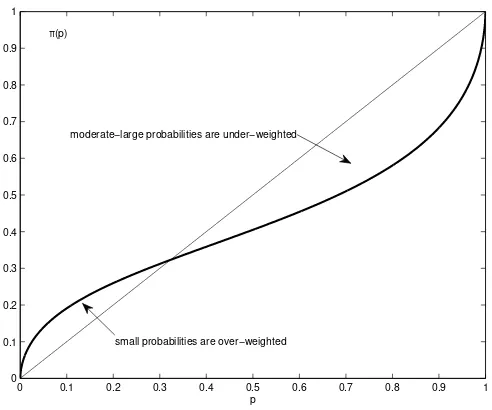
The other important idea in CPT is the notion of probability distortion:
people overweight very small probabilities and underweight average and large ones. This probability transformation is mathematically described by means
of a weighting function, that is a strictly increasing function π∶[0; 1]→[0; 1] satisfying the conditionsπ(0)=0,π(1)=1. A typical inverse S-shape weighting
function graph is shown in Figure 2.
If in CPT two different weighting functions have the role to transform the
probabilities attached to gains and losses, in our model we have a two-variables bi-weighting function. This has, in the first argument the probability of a gain
with a utility greater or equal than a given levelLand in the second argument
the probability of a symmetric loss, which utility is not smaller than −L. The
1
0 0.1 0.2 0.3 0.4 0.5 0.6 0.7 0.8 0.9 1 0
0.1 0.2 0.3 0.4 0.5 0.6 0.7 0.8 0.9 1
p
π(p)
[image:7.595.188.434.139.344.2]small probabilities are over−weighted moderate−large probabilities are under−weighted
Figure 2: CPT weighting function
final result is a number within the closed interval[−1; 1]. Formally, let us set
A ={(p, q)∈[0; 1]×[0; 1]such thatp+q≤1},
that is, in the p−q plane, the triangle which vertexes areO≡(0,0),P ≡(1,0) andQ≡(0,1).
Definition 1. We define bi-weighting function any function
ω(p, q)∶ A→[−1; 1]
satisfying the following coherence conditions:
• ω(p, q)is increasing in pand decreasing inq (bi-monotonicity)
• ω(1,0)=1,ω(0,1)= −1 andω(0,0)=0.
LetP =(x1, p1;...;xn, pn) be a lottery assigning the outcome xj ∈R with
probabilitypj, a utility functionu(⋅)∶R→R, two weighting functions π− , π+
and a bi-weighting functionω. Using an integral representation we can represent
CPT and bCPT respectively as
VCPT(P)=∫
+∞
0 π+
⎛ ⎝i∶u(∑xi)≥t
pi⎞
⎠dt −∫
+∞
0 π−
⎛
⎝i∶u(∑xi)≤−t
pi⎞
VbCPT(P)=∫
+∞
0 ω
⎛ ⎝i∶u(∑xi)≥t
pi, ∑ i∶u(xi)≤−t
pi⎞
⎠dt (2)
In our opinion, both these integrals genuinely generalize the original PT of Kahneman and Tversky (1979), preserving the main features of the theory. The
only difference is that, in (1) we get a separate evaluation of gains and losses, whereas in (2) we get a conjoint evaluation. As we will soon see, the two formulas
coincide in a non-mixed context, i.e. when the outcomes involved in the choice process are only gains or only loss. However, in the mixed case the two formulas
can differ.
3
The bi-weighting function
In this section we propose some generalizations of well known weighting
func-tions. They coincide with the original gain weighting function, π+, ifq=0, and with the opposite loss weighting function,−π−, ifp=0 .
3.1
The Kahneman-Tversky bi-weighting function
The first and most famous weighting function was proposed in Tversky and Kahneman (1992):
π(p)= p
γ
[pγ+(1−p)γ]γ1
The parameterγ can be chosen differently for gains and losses and the authors estimatedγ=0.61 for gains andγ=0.69 for losses. For this weighting function
we propose the following bipolar form
ω(p, q)= p
γ−qδ
[pγ+(1−p)γ]γ1 +[qδ+(1−q)δ]
1
δ −1
(3)
As the original KT weighting function is non monotonic for γ too much near
to zero, - see Rieger and Wang (2006), Ingersoll (2008) - so it is the case of (3) whenγandδare near zero. Proposition 1 establishes the parameter limitations
preserving the bi-monotonicity of (3). The proof is presented in appendix.
Proposition 1. The Kahneman, Tversky bi-weighting function with parameters
authors α γ
Tversky and Fox (1995) 0.77 0.79 Wu and Gonzalez (1996) 0.84 0.68 Gonzalez and Wu (1999) 0.77 0.44 Abdellaoui (2000) (gains) 0.65 0.60 Abdellaoui (2000) (losses) 0.84 0.65 Bleichrodt and Pinto (2000) 0.816 0.550
Table 1: recent estimations of parameters for the (4)
3.2
The Latimore, Baker and Witte bi-weighting function
Lattimore et al. (1992) and Goldstein and Einhorn (1987) introduced the
fol-lowing weighting function (with γ, α>0) :
π(p)= αp
γ
αpγ+(1−p)γ (4)
It is known aslinear in log odd form, since Gonzalez and Wu (1999) proved this property. We propose the following bipolar form:
ω(p, q)= α(p
γ−qδ)
αpγ+(1−p)γ+αqδ+(1−q)δ−1 (5)
Proposition 2 (proof in appendix) establishes the parameter limitations allowing for the bi-monotonicity of (5). These limitations include many of previous
parameter estimations given for the (4) (see table 1, from Bleichrodt and Pinto (2000)).
Proposition 2. The Latimore, Baker and Witte bi-weighting function with
α>1/2 and0<γ, δ≤1, is increasing in p and decreasing in q.
3.3
The Prelec bi-weighting function
One of the most famous alternative to the classical weighting function of Tversky and Kahneman (1992) is thecompound-invariant form of Prelec (1998):
π(p)=e−β(−Lnp)α (6)
where β ≈ 1 is variable for gains and for losses and 0 < α < 1. The Prelec
value of zero. We propose the following bi-weighting form:
ω(p, q)=⎧⎪⎪⎨⎪⎪
⎩
pγ−qδ ∣pγ−qδ∣e−
β(−ln∣pγ−qδ∣)α
∀(p, q)∈ A∣ pγ−qδ≠0
0 ∀(p, q)∈ A∣ pγ−qδ=0 (7)
The term ∣ppγγ−−qqδδ∣ gives±1, respectively within the OBAor OBC “triangle” of
figure 4. The (7) is extended by continuity when pγ −qδ = 0. Moreover the two parametersγ andδhave the obvious motivation that we do not wish that
ω(p, p)=0 necessarily. Note that ∣pγ−qδ∣∈[0,1]and then the logarithm is non positive. Proposition 3 establishes the parameters limitations allowing for the bi-monotonicity of (7). Without loss of generality, in the proof (see appendix)
we chooseβ=1.
Proposition 3. The Prelec bi-weighting function with β ≅ 1, γ, δ > 0 and
0<α<1 is increasing in p and decreasing in q.
3.4
The inverse S-shape of the bi-weighting function
A typical feature of the weighting function described in Tversky and Kahneman
(1992) is the inverse S-shape in the plane. Let us consider and plot the bi-polarized form of the KT weighting function, preserving the original parameters
estimationγ=.61 andδ=.69
ω(p, q)= p
0.61
−q0.69
[p0.61+(1−
p)0.61]0.161 +[
q0.69+(1−
q)0.69]0.169−1
(8)
The typical inverse S-Shape is generalized from the plane to the space (see
Figure 3). Clearly we are interested to the part of this plot such thatp+q≤1.
3.5
Stochastic dominance and bCPT
The bi-monotonicity of the bi-weighting function, ensures the bCPT model
sat-isfiesStochastic Dominance Principle. This means that, if prospect P stochas-tically dominates prospectQ, thenVbCP T(P)≥VbCP T(Q). The following
the-orem establishes this result.
Theorem 1. Let us suppose that prospects are evaluated with the bipolar CPT. Then Stochastic Dominance Principle is satisfied.
Proof. Let us consider two lotteries P = (x1, p1;x2, p2;. . .;xn, pn) and Q =
Figure 3: bi-CPT weighting function
that for allt∈R
∑
i∶xi≥t
pi≥ ∑ i∶yi≥t
qi or equivalently ∑ i∶xi≤t
pi≤ ∑ i∶yi≤t
qi (9)
By the stochastic dominance ofP overQ, we have that for allt∈R+
∑
i∶u(xi)≥t
pi≥ ∑ i∶u(yi)≥t
qi and ∑
i∶u(xi)≤−t
pi≤ ∑ i∶u(yi)≤t
qi (10)
From (10), considering the monotonicity of ω(⋅,⋅), we have that for allt∈R+
ω⎛
⎝i∶u(∑xi)≥t
pi, ∑ i∶u(xi)≤−t
pi⎞
⎠≥ω ⎛ ⎝i∶u(∑yi)≥t
qi, ∑ i∶u(yi)≤−t
qi⎞
⎠ (11)
and by monotonicity of the integral we conclude that VbCP T(P)≤VbCP T(Q).
On the other hand, in absence of the bi-monotonicity of the bi-weighting function we are able to build preferences violating the stochastic dominance. In
decreasing inq], i.e. that there exist(p, q),(̃p,q̃)∈[0,1]2
such that
⎧⎪⎪⎪⎪ ⎪⎪⎪⎪⎪ ⎨⎪⎪⎪ ⎪⎪⎪⎪⎪ ⎪⎩
p≥p̃
q≤̃q
(p−p̃)2
+(q−̃q)2
>0
ω(p, q)<ω(̃p,q̃)
Let us consider x>0 andy <0 such that u(x)=−u(y) and the two lotteries
R = (x, p;y, q) and S = (x,̃p;y,̃q). Even if R stochastically dominates S, it
would results
VbCP T(R)=ω(p, q)⋅u(x)<ω(̃p,̃q)⋅u(x)=VbCP T(S).
4
The relationship between CPT and bCPT
Given a bi-weighting function,ω(p, q)∶A→[−1; 1], it is straightforward to note that we can define two weighting functions by setting for all p, q∈[0,1]
π+(p)=ω(p,0)∶[0,1]→[0,1]
π−(q)=−ω(0, q)∶[0,1]→[0,1]
On the converse, given two weighting functions π+(p) and π−(q) we obtain a
separable bi-weighting function by setting for all(p, q)∈ A
ω(p, q)=π+(p)−π−(q)∶A→[−1; 1]
The next two propositions formalize the relationship between the two models.
Proposition 4. For non mixed prospects (containing only gains or losses) the bCPT model coincides with the CPT model.
Proof. Let us suppose that prospects are evaluated with bCPT and let u(⋅)∶
R→Rbe the utility function andω(p, q)∶A→[−1,1]the bi-weighting function. Define the two weighting function π+(p)=ω(p,0)and π−(q)=−ω(0, q)for all
p, q∈[0,1]. LetP=(x1, p1;...;xn, pn)be a prospect assigning the non-negative
outcomexj∈R+ with probabilitypj, we get:
VbCPT(P)=∫
+∞
0 ω
⎛ ⎝i∶u(∑xi)≥t
pi , ∑ i∶u(xi)≤−t
pi⎞
= ∫0+∞ω⎛
⎝i∶u(∑xi)≥t
pi, 0⎞
⎠dt = ∫
+∞
0 π+
⎛ ⎝i∶u(∑xi)≥t
pi⎞
⎠dt=VCPT(P)
In the same manner, if P =(x1, p1;...;xn, pn)is a prospect assigning the
non-positive outcome xj ∈ R− with probability pj, using ω(0, q)= −π−(q) we get
VbCPT(P)=VCPT(P). Now let us suppose that prospects are evaluated with
the CPT model and let us indicate with u(⋅) ∶ R → R the utility function
and with π+(p), π−(q)the two weighting functions. By using the bi-weighting
function ω(p, q)=π+(p)−π−(q)and replacing the steps in the above proof we getVCPT(P)=VbCPT(P).
Proposition 4 states that CPT and bCPT are the same model for non-mixed prospects. This fact is, for us, of great importance, since CPT has been widely
tested in situations involving only gains or only losses, as remembered for in-stance in Wu and Markle (2008): “In the last 50 years, a large body of
empiri-cal research has investigated how decision makers choose among risky gambles. Most of these findings can be accommodated by prospect theory... However, the
majority of the existing empirical evidence has involved single-domain gambles.
Proposition 5. If the prospects are evaluated with the bCPT model with a sepa-rable bi-weighting function, then the representation coincides with that obtained with the CPT model. On the converse, if the prospects are evaluated with the
CPT model, than the representation coincides with that obtained with the bCPT model with a separable bi-weighting function.
Proof. Let us suppose that prospects are evaluated with the bCPT model, with a separable bi-weighting function ω(p, q)=π+(p)−π−(q)∶A→[−1; 1]. We get
immediately:
VbCPT(P)=∫
+∞
0 ω⎛
⎝i∶u(∑xi)≥t
pi , ∑ i∶u(xi)≤−t
pi⎞
⎠dt=
=∫ +∞
0 π+
⎛ ⎝i∶u(∑xi)≥t
pi⎞
⎠ − π−⎛⎝ ∑
i∶u(xi)≤−t
pi⎞
⎠dt =VCPT(P)
The converse is trivially obtained reversing the above steps.
Proposition 5 establishes that CPT can be considered a special case of bCPT,
provided that we use a separable bi-weighting function. In other words there exists a (separable) bi-weighting function ω(p, q) = π+(p)−π−(q) such that
provide a preference foundation for the model, since bCPT will need a less
restrictive set of axioms with respect to CPT.
4.1
BCPT and the Wu-Markle paradox
Let us reconsider the Wu-Markle paradox described in the introduction. The paradox consists in the GLS violation, contrary to the prediction of CPT. Wu
and Markle (2008) suggested to use the same model, CPT, with a different parametrization for mixed prospects and those involving only gains or losses:
“Our study indicates that mixed gamble behavior is described well by an S-shaped utility function and an inverse S-shaped probability weighting function.
How-ever, gain-loss separability fails, and hence different parameter values are needed for mixed gambles than single-domain gambles... ”
Despite these conclusions, we are able to explain their paradox using bCPT, without changing the parameters in the passage from non mixed prospects to
mixed ones. If we use the bCPT with the bi-polarized KT weighting functions:
ω(p, q)= p
0.61
−q0.69
[p0.61+(1−
p)0.61]0.161 +[
q0.69+(1−
q)0.69]0.169−1
and the classical KT power utility function2
u(x)=⎧⎪⎪⎨⎪⎪
⎩
x.88
ifx≥0
−2.25∣−x∣.88 ifx<0
we obtain
VbCP T(H)=−443.24 > VbCP T(L)=−453.76
VbCP T(H+)=649.19 < VbCP T(L+)=652.26
VbCP T(H−)=−1,172.45 < VbCP T(L−)=−1,083.04
These results agree with the preference relation ≿. Wu and Markle (2008) is
the most influential paper showing systematic violation of GLS. Similar results are, for example, in Birnbaum and Bahra (2007). In the appendix 2 we show in detail how bCPT seems to naturally capture the essence of the phenomenon.
2
5
Extension of bCPT to uncertainty
5.1
Bi-capacity and the bipolar Choquet integral
In order to extend bCPT to the field of uncertainty, we need to generalize the concept of capacity and Choquet integral with respect to a capacity. Let
S be a non-empty set of states of the world and Σ an algebra of subsets of
S (the events). Let B denote the set of bounded real-valued Σ−measurable
functions on S and B0 the set of simple (i.e. finite valued) functions in B. A
function ν∶Σ→[0,1]is a normalized capacity on Σ if ν(∅)=0, ν(S)=1 and
ν(A)≤ν(B)wheneverA⊆B. Choquet (1953) defined an integration operation
with respect to ν. Given a nonnegative valued function f ∈B and a capacity
ν∶Σ→[0,1], the Choquet integral off with respect toν is
∫Sf(s)dν=∶∫ ∞
0
ν({s∈S∶f(s)≥t})dt
Successively Schmeidler (1986) extended this definition to all ofB:
∫Sf(s)dν=∶∫
0
−∞[ν({s∈S∶f(s)≥t})−1]dt+∫ ∞
0 ν({s∈S
∶f(s)≥t})dt
Let us consider the set of all the couples of disjoint events
Q={(A, B)∈2S×2S∶A∩B=∅}
Definition 2. A function µb∶ Q→[−1,1] is a bi-capacity onS if
• µb(∅,∅)=0,µb(S,∅)=1 andµb(∅, S)=−1
• µb(A, B)≤µb(C, D)for all(A, B),(C, D)∈Qsuch that A⊆C∧B⊇D
Grabisch and Labreuche (2005a,b); Greco et al.(2002)
Definition 3. The bipolar Choquet integral of a simple function f ∈ B0 with
respect to a bi-capacity µb is given by:
∫Sf(s)dµb=∶∫
∞
0
µb({s∈S∶f(s)>t},{s∈S∶f(s)<−t})dt
5.2
Two different approaches
Since we are working with simple acts f ∈B0, it follows that an uncertain act
can be expressed as a vector f = (x1, s1;⋯;xn, sn), wherexi will be obtained
if the state si will occur. Let f+ be the positive part of f, i.e. f+(s)=f(s)if
f(s)≥0 andf+(s)=0 if f(s)<0; similarlyf−indicates the negative part off.
The dual capacity of a capacityν∶Σ→[0,1]is defined asν̂(A)=1−ν(Ac)for
allA∈Σ. Let be given an utility functionu(⋅)∶R→R, two capacities (one for
gains, one for losses) ν+∶ S → [0,1]and ν−∶ S → [0,1]and and a bi-capacity
µb∶ Q→[−1,1].The evaluation off =(x1, s1;⋯;xn, sn)in CPT and bCPT is
VCP T(f)=∫
Su[f+(s)]dν+
+ ∫
Su[f−(s)]d̂ν−=
=∫ ∞
0
ν+({sj∶u(xj)≥t})dt−∫
0
−∞ν−({si∶u((xi)≤t})dt (12)
VbCPT(P)=∫
Su[f(s)]dµb=∫
+∞
0
µb({si∶u(xi)>t},{si∶u(xi)<−t})dt
(13)
In CPT we sum the Choquet integral of u(f+) with respect to ν+ with the Choquet integral ofu(f−) with respect toν̂−, by getting a separate evaluation
of gains and losses. In bCPT we calculate the bipolar Choquet integral ofu(f)
with respect to µb getting a conjointly evaluation of gains and losses.
5.3
Link between CPT and bCPT
As in a risk-context, the two situations where the two model coincide will occur
for non mixed acts or by using a separable bi-capacity. If µb ∶ Q→[−1,1]is a
bi-capacity, then we can define two capacitiesν+andν−as follows: for allE∈Σ
ν+(E)=µb(E,∅)
ν−(E)=−µb(∅, E)
Iff ∈B0is such thatf(s)≥0 for alls∈S, then
∫Sf(s)dµb=∫
∞
0
µb({s∈S∶f(s)>t}, ∅ )dt=
=∫ ∞
0
ν+({s∈S∶f(s)>t})dt=∫
Iff ∈B0is such thatf(s)≤0 for alls∈S, then
∫Sf(s)dµb=∫
∞
0 µb(
∅, {s∈S∶f(s)<−t})dt=
=−∫ ∞
0 ν−({s∈S
∶f(s)<−t})dt=∫
S(f(s) )d̂ν−
We have established the following important relationship between CPT and
bCPT:
Proposition 6. For non-mixed acts, the bCPT model coincides with the CPT model.
On the other hand, let us consider two capacitiesν+∶ S→[0,1]andν−∶ S→
[0,1]. Aseparable bi-capacity is defined by setting for all(A, B)∈Q
µb(A, B)=ν+(A)−ν−(B)
Proposition 7. The bCPT model with a separable bi-weighting function coin-cides with the CPT model.
In fact, the bipolar Choquet integral with respect to a separable bi-capacity is the sum of two Choquet integrals. Let f ∈ B0 be a simple function and
µb(A, B)=ν+(A)−ν−(B)a separable bi-weighting function, we get
∫Sf(s)dµb=∶∫
∞
0
µb({s∈S∶f(s)>t},{s∈S∶f(s)<−t})dt=
=∫ ∞
0 [ν+({s∈S
∶f(s)>t})−ν−({s∈S∶f(s)<−t})dt]=
=∫ ∞
0 ν+({s∈S
∶f(s)>t})dt − ∫ ∞
0 ν−({s∈S
∶f(s)<−t})dt=
∫Sf+(s)dν+ + ∫
Sf−(s)d̂ν−
In the remaining part of this paper we will face the problem of the preference
foundation of bCPT. As we have just seen, the main concept to extend bCPT from the field of risk to that of uncertainty is the bipolar Choquet integral with respect to a bi-capacity. We will present a fairly simple characterization of the
6
The characterization theorem
In this section, we first remark that the bipolar Choquet integral can be regarded as an extension of the bi-capacity. Next, we give the concept of absolutely
co-monotonic and co-signed acts, which are the special acts for which the functional is additive. Finally, we will state our main result, i.e. the characterization
theorem.
Let us identify(A, B)∈Qwith the bipolar-indicator function(A, B)∗∈B0
(A, B)∗(s)=⎧⎪⎪⎪⎪⎪⎨
⎪⎪⎪⎪⎪ ⎩
1 ifs∈A
−1 ifs∈B
0 ifs∉A∪B
Since
∫S(A, B)
∗µ
b=∫
1
0 µb(A, B)dt=µb(A, B)
then, the functional ∫Sµb, i.e. the bipolar Choquet integral, can be considered as an extension of the bi-capacityµb from QtoB0.
Definition 4. f, g∶ S→Rare absolutely co-monotonic and cosigned (a.c.c.) if
• their absolute values are co-monotonic, i.e.
( ∣f(s)∣−∣f(t)∣ )⋅( ∣g(s)∣−∣g(t)∣ )≥0 ∀s, t∈S
• they are co-signed, i.e.
f(s)⋅g(s)≥0 ∀s∈S
Let us suppose that µb is a bi-capacity and let us indicate with I(f) =
∫Sf(s)µb the bipolar Choquet integral of f with respect to µb. The next proposition lists the properties of I, and the following Theorem 2 character-izesI. Given to the importance of this section, the proofs are presented in the
main text.
Proposition 8. The functional I satisfies the following properties
• (P1) Monotonicity.
• (P2) Positive homogeneity. For alla>0, andf, a⋅f ∈B0
I(a⋅f)=a⋅ I(f);
• (P3) Bipolar-idem-potency. For allλ>0
I(λ(S,∅)∗)=λ and I(λ(∅,S)∗)=−λ;
• (P4) Additivity for acts a.c.c. Iff, g∈B0 are a.c.c., then
I(f+g)=I(f)+ I(g).
Proof. Supposingf(s)≥g(s)for alls∈S, then{s∶f(s)>t}⊇{s∶g(s)>t}and {s∈S∶f(s)<−t}⊆{s∈S∶g(s)<−t}such that (P1) follows from monotonicity of bicapacity and integral.
For alla>0 and for allf ∈B0, af∈B0, takingt=az, by definition we get
I(af)=∫ ∞
0 µb({s∈S
∶f(s)> t
a},{s∈S∶f(s)<− t a})dt=
∫0∞µb({s∈S
∶f(s)>z},{s∈S∶f(s)<−z})adz=aI(f).
which is (P2).
Forγ>0, by homogeneity,I(γ(S,∅)∗)=γI(S,∅)∗=γµb(S,∅)=γ.
If γ < 0, then I(γ(S,∅)∗) = −γI(∅, S)∗ = −γµb(∅, S) = γ. Note also that
I(0(S,∅)∗) = I((∅,∅)∗) = µb(∅,∅) = 0. Since I(λ(∅, S)∗) = −λ can be
obtained analogously, thus (P3) is proved.
Letf, g∈B0be two acts a.c.c., then, generalizing remark 4 in Schmeidler (1986), there exist
• a partition of S into k pairwise disjoint subsets ofS, (Ei)k
i=1, such that
for eachEi there existEi+andEi− withEi+∪Ei−=Ei andEi+∩E−i =∅
• twok-list of numbers 0≤α1≤α2≤⋅ ⋅ ⋅≤αk and 0≤β1≤β2≤⋅ ⋅ ⋅≤βk
such that
f =
k
∑
i=1
αi(Ei+, Ei−)
∗
, g=
k
∑
i=1
βi(Ei+, Ei−)
∗
It follows that
f+g=
k
∑
i=1
(αi+βi)(Ei+, E−i)
By the definition of bipolar Choquet integral,
I(f+g)=I(f)+I(g)
Theorem 2. Let J ∶ B0→Rsatisfy
• J((S,∅)∗)=1 andJ((∅, S)∗)=−1;
• (P1) Monotonicity;
• (P4) Additivity for acts a.c.c.;
then, by assumingµb(A, B)=J[(A, B)∗] ∀(A, B)∈Q, we have
J(f)=I(f)=∫
Sf(s)dµb
∀f ∈B0.
Proof. Let f ∈ B0 be a simple function with image f(S) = {x1, x2, . . . , xn}.
Let (⋅)∶ N → N be a permutation of indexes in N = {1,2, . . . , n} such that ∣x(1)∣≤∣x(2)∣≤⋅ ⋅ ⋅≤∣x(n)∣. f can be written as sum of double-indicator functions,
i.e.
f=
n
∑
i=1
(∣x(i)∣−∣x(i−1)∣) (A(f)(i), B(f)(i))
∗
where A(f)(i) ={s∈S∶ f(s)≥∣x(i)∣}, B(f)(i) ={s∈S∶ f(s)≤−∣x(i)∣} and
∣x(0)∣=0.
Observe that the simple functions (A(f)(i), B(f)(i))∗ for i = 1,2, . . . , n are
a.c.c., as well as the simple functions (∣x(i)∣−∣x(i−1)∣) (A(f)(i), B(f)(i))
∗
for
i=1,2, . . . , n. On the basis of this observation, applying (P4), homogeneity and
the definition ofµb(A, B)we get the thesis as follows:
J(f)=J[
n
∑
i=1
(∣x(i)∣−∣x(i−1)∣)(A(f)(i), B(f)(i))
∗
]=
=∑n
i=1
J[(∣x(i)∣−∣x(i−1)∣)(A(f)(i), B(f)(i))∗]=
=∑n
i=1
(∣x(i)∣−∣x(i−1)∣)J[(A(f)(i), B(f)(i))
∗
]=
=∑n
i=1
(∣x(i)∣−∣x(i−1)∣)µb(A(f)(i), B(f)(i))=∫
Remark 1. The properties (P2), i.e. the positive homogeneity, (P3) the bipo-lar idem-potency, are not among the hypothesis of Theorem 2 since they are
implied by additivity for absolutely co-monotonic and cosigned acts (P4) and monotonicity (P1).
Remark 2. The fact that the functional, I, is additive for a.c.c. functions, means that in the bCPT model the weakened version of independence axiom will
be true for a.c.c. acts.
7
Separating tastes from beliefs
7.1
Coherence conditions.
The bipolar Choquet integral should represent preference under uncertainty. In this case it is reasonable to expect that there is some belief about plausibility of
events A⊆S that should not depend on what is gained or lost in other events.
In this context it is reasonable to imagine that the value given by a bi-capacity
µb to(A, B)∈Qis not decreasing with the plausibility ofAand non-increasing
with the plausibility of B. If this is true, then one has to expect that should
not be possible to haveµb(A, C)>µb(B, C)andµb(A, D)<µb(B, D). In fact,
this would mean that act(A, C)∗ would be preferred to act(B, C)∗, revealing
a greater credibility of A over B, and act (A, D)∗ would be preferred to act (B, D)∗, revealing a greater credibility of B over A. Similar situations arise when µb(C, A)> µb(C, B) and µb(D, A)< µb(D, B), or µb(A, C)> µb(B, C)
andµb(D, A)>µb(D, B). Taking into account such situations, we shall analyze
in detail the following coherence conditions:
(A1) (A, C)∗≻(B, C)∗⇒(A, D)∗≻(B, D)∗, for all(A, C),(B, C),(A, D),(B, D)∈Q, (A2) (C, A)∗≻(C, B)∗⇒(D, A)∗≻(D, B)∗,
for all(C, A),(C, B),(D, A),(D, B)∈Q,
(A3) for anyA, B⊆S there exist oneC⊆S∖(A∪B)such that
(A, C)∗≻(B, C)∗⇔(C, A)∗≺(C, B)∗
(A4) (A, C)∗≻(B, C)∗⇔(C, A)∗≺(C, B)∗, for all(A, C),(B, C),(C, A),(C, B)∈Q, (A5) (A, C)∗≻(B, C)∗⇔(D, A)∗≺(D, B)∗,
Theorem 3. The following proposition hold
1) If (A1) holds, then there exists a capacity ν1 on S and a function
ω1∶{(v, B)∶v=ν1(A),(A, B)∈Q}→[−1,1],
such thatµb(A, B)=ω1(ν1(A), B)for all(A, B)∈Q, with functionω1
in-creasing in the first argument and non inin-creasing with respect to inclusion
in the second argument;
2) If (A2) holds, then there exists a capacity ν2 on S and a function
ω2∶{(A, v)∶v=ν2(B),(A, B)∈Q}→[−1,1],
such thatµb(A, B)=ω2(A, ν2(B))for all(A, B)∈Q, with functionω2non
decreasing with respect to inclusion in the first argument and decreasing in the second argument;
3) If (A1) and (A2) hold, then there exist two capacities ν1 andν2 onS and a function
ω3∶{(u, v)∶u=ν1(A), v=ν2(B),(A, B)∈Q}→[−1,1],
such that µb(A, B)=ω3(ν1(A), ν2(B)) for all (A, B)∈Q, with function ω3increasing in the first argument and decreasing in the second argument;
4) If (A1), (A2) and (A3) hold, then there exists a capacity ν on S and a
function
ω∶{(u, v)∶u=ν(A), v=ν(B),(A, B)∈Q}→[−1,1],
such that µb(A, B)= ω(ν(A), ν(B)) for all (A, B)∈ Q, with function ω
increasing in the first argument and decreasing in the second argument;
5) If (A1) and (A4) hold, then there exists a capacity ν on S and a function
ω∶{(u, v)∶u=ν(A), v=ν(B),(A, B)∈Q}→[−1,1],
such that µb(A, B)= ω(ν(A), ν(B)) for all (A, B)∈ Q, with function ω
6) If (A2) and (A4) hold, then there exists a capacity ν onS and a function
ω∶{(u, v)∶u=ν(A), v=ν(B),(A, B)∈Q}→[−1,1]
such that µb(A, B)= ω(ν(A), ν(B)) for all (A, B)∈ Q, with function ω
increasing in the first argument and decreasing in the second argument;
7) If (A5) holds, then there exists a capacity ν onS and a function
ω∶{(u, v)∶u=ν(A), v=ν(B),(A, B)∈Q}→[−1,1],
such that µb(A, B)= ω(ν(A), ν(B)) for all (A, B)∈ Q, with function ω
increasing in the first argument and decreasing in the second argument.
The proof is presented in appendix 3.
8
Concluding Remarks
In bCPT, gains and losses within a mixed prospect are evaluated conjointly and not separately, as in CPT. This permits to account for situations in which
CPT fails, due to gain-loss separability, such as the “Wu-Markle paradox”. In this paper we propose a natural generalization of CPT, which, fundamentally:
a) totally preserve CPT in non-mixed cases; b) allows for GLS violation in mixed case. The main concept to get an axiomatic foundation of bCPT, in
decision under uncertainty, is the bipolar Choquet integral, about which, we have presented a fairly simple characterization. A full axiomatization of the
model, in terms of preferences foundation, will be the aim for future researches.
References
Abdellaoui, M. (2000). Parameter-free elicitation of utility and probability
weighting functions. Management Science,46(11), 1497–1512.
Allais, M. (1953). Le comportement de l’homme rationnel devant le risque:
Cri-tique des postulats et axiomes de l’´ecole Am´ericaine. Econometrica: Journal of the Econometric Society, 21(4), 503–546.
prospect theory in mixed gambles with moderate probabilities. Management
Science,52(8), 1288.
Barberis, N., Huang, M., and Santos, T. (2001). Prospect Theory and Asset
Prices. Quarterly Journal of Economics, 116(1), 1–53.
Benartzi, S. and Thaler, R. (1995). Myopic loss aversion and the equity premium
puzzle. The Quarterly Journal of Economics, 110(1), 73–92.
Birnbaum, M. (2005). Three new tests of independence that differentiate models
of risky decision making. Management Science,51(9), 1346–1358.
Birnbaum, M. and Bahra, J. (2007). Gain-loss separability and coalescing in
risky decision making. Management Science,53(6), 1016–1028.
Blavatskyy, P. (2005). Back to the St. Petersburg paradox? Management
Science,51(4), 677–678.
Bleichrodt, H. and Pinto, J. (2000). A parameter-free elicitation of the
proba-bility weighting function in medical decision analysis. Management Science,
46(11), 1485–1496.
Camerer, C. (2000). Prospect theory in the wild: Evidence from the field.
Advances in Behavioral Economics.
Choquet, G. (1953). Theory of capacities. Ann. Inst. Fourier,5(131-295), 54.
Ellsberg, D. (1961). Risk, ambiguity, and the Savage axioms. The Quarterly
Journal of Economics, 75(4), 643–669.
Gilboa, I. (1987). Expected utility with purely subjective non-additive
proba-bilities. Journal of Mathematical Economics,16(1), 65–88.
Goldstein, W. and Einhorn, H. (1987). Expression theory and the preference
reversal phenomena. Psychological Review,94(2), 236.
Gonzalez, R. and Wu, G. (1999). On the shape of the probability weighting
function. Cognitive Psychology, 38(1), 129–166.
Grabisch, M. and Labreuche, C. (2005a). Bi-capacities–I: definition, M
”obius transform and interaction. Fuzzy sets and systems,151(2), 211–236.
Grabisch, M. and Labreuche, C. (2005b). Bi-capacities–II: the Choquet integral.
Greco, S., Matarazzo, B., and Slowinski, R. (2002). Bipolar Sugeno and Choquet
integrals. InEUROFUSE Workshop on Informations Systems, pages 191–196.
Ingersoll, J. (2008). Non-monotonicity of the Tversky-Kahneman
probability-weighting function: a cautionary note. European Financial Management,
14(3), 385–390.
Jolls, C., Sunstein, C., and Thaler, R. (1998). A behavioral approach to law and economics. Stanford Law Review, 50(5), 1471–1550.
Kahneman, D. and Tversky, A. (1979). Prospect theory: An analysis of decision under risk. Econometrica: Journal of the Econometric Society, 47(2), 263– 291.
Lattimore, P., Baker, J., and Witte, A. (1992). The influence of probability on
risky choice:: A parametric examination. Journal of Economic Behavior & Organization,17(3), 377–400.
Levy, M. and Levy, H. (2002). Prospect Theory: Much ado about nothing?
Management Science,48(10), 1334–1349.
Luce, R. (1999). Binary Gambles of a Gain and a Loss: an Understudied Do-main. Mathematical utility theory: utility functions, models, and applicaitons
in the social sciences, 8, 181–202.
Luce, R. (2000). Utility of Gains and Losses:: Measurement-Theoretical, and
Experimental Approaches.
McNeil, B., Pauker, S., Sox Jr, H., and Tversky, A. (1982). On the elicitation
of preferences for alternative therapies. New England journal of medicine,
306(21), 1259–1262.
Prelec, D. (1998). The probability weighting function. Econometrica, 66(3), 497–527.
Quattrone, G. and Tversky, A. (1988). Contrasting rational and psychological analyses of political choice. The American political science review, 82(3), 719–736.
Quiggin, J. (1982). A theory of anticipated utility. Journal of Economic
Rieger, M. and Wang, M. (2006). Cumulative prospect theory and the St.
Petersburg paradox. Economic Theory, 28(3), 665–679.
Schade, C., Schroeder, A., and Krause, K. (2010). Coordination after gains and
losses: Is prospect theory’s value function predictive for games? Journal of
Mathematical Psychology.
Schmeidler, D. (1986). Integral representation without additivity. Proceedings of the American Mathematical Society, 97(2), 255–261.
Schmeidler, D. (1989). Subjective probability and expected utility without ad-ditivity. Econometrica: Journal of the Econometric Society,57(3), 571–587.
Tversky, A. and Fox, C. (1995). Weighing risk and uncertainty. Psychological review,102(2), 269–283.
Tversky, A. and Kahneman, D. (1992). Advances in prospect theory: Cumu-lative representation of uncertainty. Journal of Risk and uncertainty, 5(4), 297–323.
Von Neumann, J. and Morgenstern, O. (1944).Theories of games and economic
behavior. Princeton University Press Princeton, NJ.
Wu, G. and Gonzalez, R. (1996). Curvature of the probability weighting
func-tion. Management Science,42(12), 1676–1690.
Wu, G. and Markle, A. (2008). An empirical test of gain-loss separability in
9
Appendix 1
Proof of proposition 1.
Forx∈[0,1]and δ ∈[0,1] it results f(x)=[xδ+(1−x)δ] 1
δ ≥1 since this
function is continuous in the closed interval [0,1], withf(0)=f(1)=1, while
f′(x)is positive in]0,1/2[and negative in]1/2,1[. In fact:
f′(x)=[xδ+(1−x)δ] 1
δ−1[
xδ−1−(1−x)δ−1]≥0
⇔ [xδ−1−(1−x)δ−1]≥0 ⇔ 1≥( x 1−x)
1−δ
⇔ x≤ 1
2
It follows that in (3) the denominator is positive and the sign depends onpγ−qδ.
If we start from the zero curveω(p, q)=0 ⇔ pγ−qδ=0, that is theOB̂ curve in figure 4 , it is clear that an increase inpwill bring us in the domain in which the function (3) is positive (OAB ”triangle”) while an increase in q will bring
us in the domain in which the function is negative (OBC ”triangle”) and then, in this case, the function (3) is increasing in p and decreasing in q. Now it is
sufficient to prove thatω(p, q)is increasing inpand decreasing inq within the two triangles, i.e. where ω(p, q)>0 (<0)and p, q>0. If ω(p, q)>0, and then ifpγ−qδ>0 and since the function ln(x)is strictly increasing, it is sufficient to
prove that ln[ω(p, q)] is increasing inpand decreasing inq. By differentiating
w. r. t. the first variable:
∂ln[ω(p, q)]
∂p =
γpγ−1 pγ−qδ −[(
1
p) 1−γ
−( 1
1−p) 1−γ
]⋅
⋅ [p
γ+(1−p)γ]γ1−1
[pγ+(1−p)γ]
1
γ +[
qδ+(1−q)δ]
1
δ −1
(14)
If 1/2 ≤ p< 1 → [(1
p)
1−γ
−(11 −p)
1−γ
] ≤ 0 and (14) is positive. Suppose 0<p<1/2, then the first summand in (14) is positive and the second is negative. We have the following decreasing sequence:
∂ln[ω(p, q)]
∂p =
γpγ−1 pγ−qδ −[(
1
p) 1−γ
−( 1
1−p) 1−γ
⋅ [p
γ+(1−p)γ]1γ−1
[pγ+(1−p)γ]
1
γ +[
qδ+(1−q)δ]
1
δ −1
≥3
≥ γpγ−
1
pγ −[(
1
p) 1−γ
−( 1
1−p) 1−γ
]⋅ [p
γ+(1−p)γ]γ1−1
[pγ+(1−p)γ]
1
γ+[qδ+(1−q)δ]
1
δ −1
≥4
≥γpγ−1
pγ −[(
1
p) 1−γ
−( 1
1−p) 1−γ
]⋅[p
γ+(1−p)γ
]γ1−1
[pγ+(1−p)γ]
1
γ =
= γpγ−
1
pγ −[(
1
p) 1−γ
−( 1
1−p) 1−γ
]⋅ 1
pγ+(1−p)γ ≥
5
≥γ(
1
p)
1−γ
pγ −
(1
p)
1−γ
pγ+(1−p)γ =(
1
p) 1−γ
⋅[γ
pγ −
1
pγ+(1−p)γ]
Now, in order to prove that the (14) is non negative, it is sufficient to show that
the quantity in the last square bracket is non negative, i.e.
γ pγ −
1
pγ+(1−p)γ =
γ[pγ+(1−p)γ]−pγ
pγ[pγ+(1−p)γ] ≥0 ⇔ γ[p
γ+(1−p)γ]−pγ ≥0
⇔ γ(1−p)γ ≥(γ)pγ ⇔ (1−p p )
γ
≥1−γ
γ ⇔
1−p p ≥(
1−γ γ )
1
γ
Remembering that we are under the limitation 0 < p < 1/2 the first term is
3
since
γpγ−1
pγ−qδ >
γpγ−1
pγ
4
since from
[qδ+ (1−q)δ]
1
δ−
1≥0→ [p
γ+(1−p)γ]1γ−1
[pγ+(1−p)γ]γ1+[qδ+(1−q)δ] 1
δ−
1
≤[pγ+(1−p)γ]
1
γ−1 [pγ+(1−p)γ]γ1 →
−⎡⎢⎢⎢
⎢⎣(
1 p)
1−γ
−( 1
1−p)
1−γ⎤⎥
⎥⎥
⎥⎦ [
pγ+(1−p)γ]
1
γ−1 [pγ+(1−p)γ]
1
γ+[qδ+(1−q)δ] 1 δ− 1 ≥ −⎡⎢⎢⎢ ⎢⎣( 1 p)
1−γ
−( 1
1−p)
1−γ⎤⎥
⎥⎥ ⎥⎦[
pγ+(1−p)γ]γ1−1
[pγ+(1−p)γ]γ1
5
since
−(1
p)
1−γ
≤ −⎡⎢⎢⎢
⎢⎣(
1 p)
1−γ
−( 1
1−p)
1−γ⎤⎥
greater than 1 and the last inequality is true if
(1−γγ)
1
γ
≤1 ⇔ γ≥ 1
2
and this is ensured by the hypothesis of proposition 1.
Thus we have proved that ifω(p, q)>0 then the functionω(p, q)is increasing in
p. An analogous proof gives that, ifω(p, q)<0, then the function is decreasing in q, i.e. the function −ω(p, q) is increasing in q. For this it is sufficient to exchange pwithq andγ withδ and to repeat the previous passages. Now, in
the caseω(p, q)>0 we turn out our attention to the first derivative of ln[ω(p, q)]
with respect to q
∂ln[ω(p, q)]
∂q =
−δqδ−1 pγ−qδ −[(
1
q) 1−δ
−( 1
1−q) 1−δ
]⋅
⋅ [
qδ+(1−q)δ]
1
δ−1
[pγ+(1−p)γ]
1
γ +[
qδ+(1−q)δ]
1
δ −1
(15)
If [(1
q)
1−δ
−( 1 1−q)
1−δ
] ≥ 0 ⇔ q ≤ 1/2 then the (15) is negative. Supposing
q>1/2, the first summand in (15) is negative and the second is positive. Note that ifγ≥δ, the curve which equation ispγ−qδ =0 coincides with the graph of
the functionq=pγδ that is convex, like in figure 4, and within the domain
A+={(p, q)∈[0; 1]×[0; 1]such thatp+q≥1 andpγ−qδ}
it is impossible that q> 1/2 and so we have finished the proof. On the other hand, ifγ<δthe graph of the functionq=pγδ is concave and within the domain
A+ there are points such that q > 1/2. For these reasons, from here we will supposeq>1/2 andγ<δ and we will refer to figure 5.
From a sequence of increases it results:
∂ln[ω(p, q)]
∂q ≤
6
≤ −δqδ−
1
pγ−qδ −[(
1
q) 1−δ
−( 1
1−q) 1−δ
] =
6
since from
1/2<γ, δ≤1 → [pγ+(1−p)γ]
1
γ−1≥0 and [qδ+(1−q)δ]
1
δ≥
1→
[qδ+(1−q)δ] 1
δ−1
[pγ+(1−p)γ] 1
γ+[qδ+(1−q)δ] 1
δ−1
≤[q
δ+(1−q)δ] 1
δ−1
[qδ+(1−q)δ] 1
δ
= 1
= qδ−1[ −δ pγ−qδ +(
q
1−q) 1−δ
−1]
Then it is sufficient to prove that
−δ pγ−qδ +(
q
1−q) 1−δ
−1 ≤ 0 ⇔ ( q
1−q) 1−δ
≤ 1+ −δ
pγ−qδ
and this will follow from:
q
1−q ≤ 1+
−δ pγ−qδ
since
q> 1
2 ⇒
q
1−q >1 ⇒ ( q
1−q) 1−δ
⇒ 1−q
q
For our scope we must prove that
q
1−q ≤ 1+
−δ
pγ−qδ (16)
Under the restrictions we are working with, it is possible to elicit some
limita-tions of the variablesp, q, γ and δ. We have supposedpγ−qδ >0 , q>1/2 and
δ>γ, that in figure 5 delimit the area ABC. Since the curvature of pγ−qδ =0 is more accentuate when larger is the difference betweenγ andδ, a limit is, for us, the curvep0.5
−q1=
0, i.e. q=√p, which delimits the area ADE containing
the area ABC. This consideration allows us to elicit some sure limitations forp
andq: the “highest” point is the intersection betweenq=√pandp+q=1, that
isD(0.38; 0.62); the most “left-placed” point is the intersection betweenq=√p
andq=0.5, that isE(0.25; 0.5); we elicit 0.25<p<0.5 and 0.5<q<0.62.
Con-sider the functionpγ−qδ, by differentiating, we can prove that it is increasing
in pand δ and decreasing in q and γ, and then, using the elicited parameter
limitations we have
pγ−qδ ≤ (1
2)
0.5
−(1
2)
1
which in turn implies
1+ −δ
pγ−qδ ≥ 1+
δ
(1 2)
0.5
−(12)1
(17)
limitation ofqit follows that
q
1−q ≤
0.62
1−0.62 (18)
Using (17) and (18) the (16) is true if it is true the:
0.62
1−0.62 ≤ 1+
δ
(1 2)
0.5
−(12)1
which givesδ>0.131 that is within our limitations. Similarly, by exchangingp
withqandγ withδit follows that ω(p, q)is increasing inpwhenω(p, q)<0.
Q.E.D.
Proof of proposition 2.
Forx∈[0,1],α>1/2 andγ∈]0,1]it resultsf(x)=αxγ+(1−x)γ≥min{1, α}>
1/2. Since this function is continuous in the closed interval[0,1], withf(0)=1,
f(1)=αand the second derivative is non-positive from zero to one:
f′′(x)=γ(γ−1)αxδ−2+γ(γ−1)(1−x)δ−2≤0
It follows that, in (5), the denominator is positive under the limitationα>1/2. Within its domain the first derivative of the (5) with respect to pis :
∂ω(p, q) ∂p =αγ
(1−p)γ−1
(pγ−1
−qδ)+pγ−1
[2αqδ+(1−q)δ−1] [αpγ+(1−p)γ+αqδ+(1−q)δ−1]
2 (19)
Having chosen γ ≤1 the term pγ−1 ≥
1 for all p∈]0,1] and since qδ ≤ 1 then
pγ−1
−qδ ≥0 . On the other hand (2αqδ+1−q)δ−1 ≥0 since for x∈ [0,1],
α>1/2 and 0<δ≤1 the functionf(x)=2αxδ+(1−x)δ≥min{1,2α}≥1 since it is continuous in the closed interval [0,1], with f(0)=1, f(1)=2αand the second derivative is non-positive from zero to one:
f′′(x)=γ(γ−1)2αxδ−2+γ(γ−1)(1−x)δ−2≤0
Then (19) is non-negative and the (5) is increasing inp.
The first derivative with respect toqis
∂ω(p, q) ∂q =αδ
(1−q)δ−1(pγ−qδ−1)−qδ−1[2αpγ+(1−p)γ−1] [αpγ+(1−p)γ+αqδ+(1−q)δ−1]
By the same argumentations, it is easy to see that it is non-positive and then
the (5) is decreasing inq.
Q.E.D.
Proof of proposition 3.
If we start from the zero curve ω(p, q) = 0 ⇔ pγ −qδ = 0 that is the OB̂
curve in figure 4, it is clear that an increasing in p will bring them in the domain in which the function is positive (OAB “triangle”) while an increasing
in q will bring them in the domain in which the function is negative (OBC
“triangle”) and, in this case, the function (7) is increasing inpand decreasing in q.Now it is sufficient to prove that ω(p, q)is increasing inpand decreasing in qwithin the two triangle, i.e. whereω(p, q)>0 orω(p, q)<0 andp, q>0.If
w(p, q)>0 and then ifpγ−qδ>0 the (7) becomes: ω(p, q)=e−[−Ln(pγ−qδ)]α
and by differentiating w. r. t. the two variables:
∂ω(p, q) ∂p =e
−[−Ln(pγ−qδ)]α
α[−Ln(pγ−qδ)]α−1 γp
γ−1 pγ−qδ >0
∂ω(p, q) ∂p =e
−[−Ln(pγ−qδ)]αα[−Ln(pγ−qδ)]α−1−δqδ−
1
pγ−qδ <0
This proves the property within the triangleOBA, whereω(p, q)>0. Similarly ifpγ−qδ<0 the (7) becomes: ω(p, q)=−e−[−Ln(−pγ+qδ)]α and by differentiating w. r. t. the two variables:
∂ω(p, q) ∂p =−e
−[−Ln(−pγ+qδ)]α
α[−Ln(pγ−qδ)]α−1 −γp
γ−1
−pγ+qδ >0
∂ω(p, q) ∂p =−e
−[−Ln(−pγ+qδ)]αα[−Ln(pγ−qδ)]α−1 δqδ−
1
−pγ+qδ <0
We conclude that the Prelec bi-weighting function is increasing in its first
argu-ment and decreasing in the second, for all the parameter values.
0 0.1 0.2 0.3 0.4 0.5 0.6 0.7 0.8 0.9 1 0
0.1 0.2 0.3 0.4 0.5 0.6 0.7 0.8 0.9 1
p=q
ω(p,q)<0
ω(p,q)>0 B C(0,1)
q
p A(1,0)
[image:33.595.161.465.144.393.2]ω(p,q)=0
Figure 4: the KT bi-weighting function domain; in the case γ > δ, the curve
q=pγ/δ is convex.
10
Appendix 2
10.1
Recent literature denouncing GLS
As discussed in the paper, this study aims to generalize CPT, allowing gains and
losses within a mixed prospect to be evaluated conjointly, rather than separately. In the following we shall focus our attention on two recent papers: Wu and
Markle (2008) and Birnbaum and Bahra (2007). Both of them report systematic violations of GLS. CPT and all the model it generalizes, such as EUT, cannot
account for such a pattern of choice. We show how bCPT is able to capture, at least partially, these errata predictions.
10.2
Wu and Markle (2008)
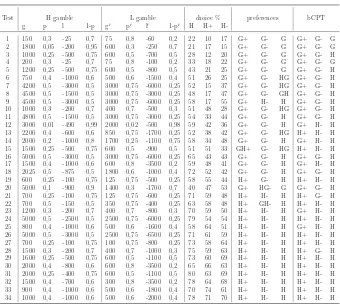
In table 2 we reproduce Table 1 of page 1326 in Wu and Markle (2008), with the preferences elicited from the reported percentages found by the authors.
In many cases (tests 6,7, 10-18) the respondents preferred (in percentage) H
part, the preferences were reversed. To test our model we have used the bCPT
functional
VbCP T(P)=∫
∞
0 ω
⎛ ⎝i∶u(∑xi)≥t
pi, ∑ i∶u(xi)≤−t
pi⎞
⎠dt (21)
based on the KT bi-weighting function
ω(p, q)= p
γ−qδ
[pγ+(1−p)γ]γ1 +[qδ+(1−q)δ]
1
δ −1
(22)
with parametersγ=0.9 andδ=0.89 and the classical KT power utility function
u(x)=⎧⎪⎪⎨⎪⎪
⎩
xα+ ifx≥0
−λ(−x)α
− ifx<0
(23)
with parametersλ=1.77 ,α+=0.68, andα−=0.79.
As can be seen in table 2, our data are in the same directions of the preferences in all the pure positive choices except that in tests 13, 23 and 25, in all the
pure negative choices except in tests 9, 12-15, 17 and 19 and in all the mixed choices except in tests 3, 5 and 20. But, what we think is very interesting, is
that bCPT is able explain the reversed preferences, totally in tests 6, 7, 10, 11, 16 and 18 and partially in test 12, 14, 15, and 17. The model seems able to
naturally capture, totally or partially, the GLH.
10.3
Birnbaum-Bahra
Birnbaum and Bahra (2007) reported systematic violations of two behavioral
properties implied by CPT. One, is the just discussed GLS and the other, is
the property known as coalescing: “coalescing is the assumption that if there are two probability-consequences branches in a gamble leading to the same con-sequence, they can be combined by adding their probabilities.” For example, the
three-branch gamble A = ($100,25%;$100,25%;$0,50%) should be equivalent to the two-branch gamble A′=($100,50%;$0,50%). Our model is not able to
accommodate for violation of coalescing, but we want some questions.
Birn-baum and Bahra tested violation of coalescing presenting to the participants the gambles in terms of a container holding exactly 100 marbles of different
colors. So, according to coalescing,B′=(25red $100; 75white $0) should be
considered equivalent toB=(25red$100; 25white$0; 50white$0). We are not
Table 2: application of bCPT to the data of Wu and Markle (2008)
Test H gamble L gamble choice % preferences bCPT g p l 1-p g′ p′ l′ 1-p′ H H+
H-1 150 0,3 -25 0,7 75 0,8 -60 0,2 22 10 17 G+ G- G G+ G- G 2 1800 0,05 -200 0,95 600 0,3 -250 0,7 21 17 15 G+ G- G G+ G- G 3 1000 0,25 -500 0,75 600 0,5 -700 0,5 28 12 20 G+ G- G G+ G- H 4 200 0,3 -25 0,7 75 0,8 -100 0,2 33 18 22 G+ G- G G+ G- G 5 1200 0,25 -500 0,75 600 0,5 -800 0,5 43 21 25 G+ G- G G+ G- H 6 750 0,4 -1000 0,6 500 0,6 -1500 0,4 51 26 25 G+ G- HG G+ G- H 7 4200 0,5 -3000 0,5 3000 0,75 -6000 0,25 52 15 37 G+ G- HG G+ G- H 8 4500 0,5 -1500 0,5 3000 0,75 -3000 0,25 48 17 47 G+ G- GH G+ G- H 9 4500 0,5 -3000 0,5 3000 0,75 -6000 0,25 58 17 55 G+ H- H G+ G- H 10 1000 0,3 -200 0,7 400 0,7 -500 0,3 51 48 28 G+ G- HG G+ G- H 11 4800 0,5 -1500 0,5 3000 0,75 -3000 0,25 54 33 44 G+ G- H G+ G- H 12 3000 0,01 -490 0,99 2000 0,02 -500 0,98 59 42 36 G+ G- H G+ H- H 13 2200 0,4 -600 0,6 850 0,75 -1700 0,25 52 38 42 G+ G- HG H+ H- H 14 2000 0,2 -1000 0,8 1700 0,25 -1100 0,75 58 34 48 G+ G- H G+ H- H 15 1500 0,25 -500 0,75 600 0,5 -900 0,5 51 51 33 GH+ G- HG H+ H- H 16 5000 0,5 -3000 0,5 3000 0,75 -6000 0,25 65 43 43 G+ G- H G+ G- H 17 1500 0,4 -1000 0,6 600 0,8 -3500 0,2 59 48 41 G+ G- H G+ H- H 18 2025 0,5 -875 0,5 1800 0,6 -1000 0,4 72 52 42 G+ G- H G+ G- H 19 600 0,25 -100 0,75 125 0,75 -500 0,25 58 55 44 H+ G- H H+ H- H 20 5000 0,1 -900 0,9 1400 0,3 -1700 0,7 40 47 53 G+ HG- G G+ G- H 21 700 0,25 -100 0,75 125 0,75 -600 0,25 71 59 48 H+ H- H H+ G- H 22 700 0,5 -150 0,5 350 0,75 -400 0,25 63 58 48 H+ GH- H H+ H- H 23 1200 0,3 -200 0,7 400 0,7 -800 0,3 70 59 50 H+ H- H G+ H- H 24 5000 0,5 -2500 0,5 2500 0,75 -6000 0,25 79 54 54 H+ H- H H+ H- H 25 800 0,4 -1000 0,6 500 0,6 -1600 0,4 58 64 51 H+ H- H G+ H- H 26 5000 0,5 -3000 0,5 2500 0,75 -6500 0,25 71 61 59 H+ H- H H+ H- H 27 700 0,25 -100 0,75 100 0,75 -800 0,25 73 58 64 H+ H- H H+ H- H 28 1500 0,3 -200 0,7 400 0,7 -1000 0,3 75 59 63 H+ H- H H+ G- H 29 1600 0,25 -500 0,75 600 0,5 -1100 0,5 73 60 69 H+ H- H H+ H- H 30 2000 0,4 -800 0,6 600 0,8 -3500 0,2 65 66 63 H+ H- H H+ H- H 31 2000 0,25 -400 0,75 600 0,5 -1100 0,5 80 63 69 H+ H- H H+ H- H 32 1500 0,4 -700 0,6 300 0,8 -3500 0,2 78 64 68 H+ H- H H+ H- H 33 900 0,4 -1000 0,6 500 0,6 -1800 0,4 70 74 61 H+ H- H H+ H- H 34 1000 0,4 -1000 0,6 500 0,6 -2000 0,4 78 71 70 H+ H- H H+ H- H
gambles with the numerical probabilities. In fact, a person facingB could ask
himself what is the reason that the first 25 white marbles were not summed to
the second 50 white marbles. It is admissible that she could think if they differ in some way, e.g. in size. In any case, she will have an additional information, or doubt to process and this could generate errors. As focused from Wu and
Markle (2008), the examples of Birnbaum and Bahra (2007) to underline the GLS violation, are less simple than theirs, but our model is able to accommodate
for these violations too. The only we need is to modify the parameterγ from
the value of 0.9, used to accommodate the majority of data in Wu and Markle (2008), to the value of 0.74. Next, we report the part of the table 5 at page 1022
in Birnbaum and Bahra (2007) that, in the words of the same authors, form a test for the GLS. Each gamble “is described in terms of a container holding
exactly 100 marbles of different colors, from which one marble would be drawn at random, and the color of that marble would determine the prize.”. In the
brackets are shown the percentages of each choose.
F= ⎛ ⎜⎜ ⎜⎜ ⎜⎜ ⎜⎜ ⎜⎜ ⎜⎜ ⎝ 25black to win$100
25white to win$0
50pink to lose$50
⎞ ⎟⎟ ⎟⎟ ⎟⎟ ⎟⎟ ⎟⎟ ⎟⎟ ⎠ ≻ ⎛ ⎜⎜ ⎜⎜ ⎜⎜ ⎜⎜ ⎜⎜ ⎜⎜ ⎝ 50blue to win$50
25white to lose$0
25red to lose$100
⎞ ⎟⎟ ⎟⎟ ⎟⎟ ⎟⎟ ⎟⎟ ⎟⎟ ⎠ =G
[76%] [24%]
F+=
⎛ ⎜⎜ ⎜⎜ ⎜⎜ ⎜⎜ ⎜⎜ ⎜⎜ ⎝ 25black to win$100
25white to win$0
50white to win$0
⎞ ⎟⎟ ⎟⎟ ⎟⎟ ⎟⎟ ⎟⎟ ⎟⎟ ⎠ ≺ ⎛ ⎜⎜ ⎜⎜ ⎜⎜ ⎜⎜ ⎜⎜ ⎜⎜ ⎝ 25blue to win$50
25blue to win$50
50white to win$0
⎞ ⎟⎟ ⎟⎟ ⎟⎟ ⎟⎟ ⎟⎟ ⎟⎟ ⎠
=G+