Munich Personal RePEc Archive
Gravity and extended gravity: estimating
a structural model of export entry
Morales, Eduardo and Sheu, Gloria and Zahler, Andrés
Harvard University
January 2011
Gravity and Extended Gravity:
Estimating a Structural Model of Export Entry
∗Eduardo Morales1, Gloria Sheu2, and Andr´es Zahler3 1Harvard University
2U.S. Department of Justice 3Harvard University
January 16th, 2011
JOB MARKET PAPER
Abstract
Exporters continuously enter and exit individual foreign markets. Although a given firm’s status as an exporter tends to be persistent, the set of destination countries that a firm serves changes frequently. In this paper we empirically examine the determinants of a firm’s choice of destination countries and show that their export paths follow systematic patterns. We develop a model of export dynamics where firms decide in each period the countries to which they sell. Our model allows profits from each possible destination country to depend on: (a) how similar it is to the firm’s home country (gravity), and (b) how similar it is to other destinations to which the firm has previously exported (extended gravity). Given the enormous number of possible export paths from which firms may choose, conventional estimation approaches based on discrete choice models are unfeasible. Instead, we use a moment inequalities approach. Our inequalities come from applying an analogue of Euler’s perturbation method to a discrete choice setting. We show that standard gravity forces have a much larger influence on sunk costs than on fixed costs of exporting and that extended gravity effects can be substantial.
JEL Classifications: F12, C51, L65
Keywords: gravity, extended gravity, export dynamics, moment inequalities
1
Introduction
Exporters continuously enter and exit individual foreign markets. Although a given firm’s status as an exporter is persistent, the specific set of countries that a firm serves changes frequently. These export dynamics generate economy-wide productivity fluctuations in the exporting countries through intra-industry resource re-allocations (Pavcnik (2002), Melitz (2003)) and within firm productivity growth coming from learning by exporting (Van Biese-broeck (2005), De Loecker (2007), Lileeva and Trefler (2010)). The entry and exit of firms in foreign markets also has direct welfare implications for importing countries as they affect the range of product varieties available for consumption (Broda and Weinstein (2006)). Besides its welfare implications, the movement of firms in and out of export markets has proved rel-evant in explaining long-run changes in aggregate trade flows (Evenett and Venables (2002), Bernard et al. (2009), Lawless (2009)), asymmetric responses to temporary and permanent changes in expected export profits (Ruhl (2008)), persistent deviations from purchasing power parity (Ghironi and Melitz (2005)), and variation in stock market returns and earnings yields (Fillat and Garetto (2010)).
This paper analyzes the determinants of firm entry and exit into foreign markets. We allow export dynamics in each potential destination country to depend on: (a) similarity between the importing country and the firm’s home country, and (b) similarity between the current importing country and prior destinations of the firm’s exports. Therefore, the model borrows from the most recent gravity equation literature the intuition that firms tend to access first markets that are larger and geographically and linguistically closer to the country of origin (e.g. Eaton and Kortum (2002), Helpman et al. (2008)). Besides, we complement this intuition by allowing export decisions of firms in every time period to also depend on their previous
exporting history. More precisely, this paper introduces the concept of extended gravity as a
new determinant of firm entry into export markets. While gravity reflects closeness between home and destination markets, extended gravity depends on similarities between two receiving countries. We quantify how strong gravity and extended gravity effects are in determining firms’ country-specific entry and exit decisions.
sources of adaptation costs may be time spent in looking for a distributor, or wages paid to newly-hired workers with specific skills (e.g. language skills). Given that adaptation costs are likely to be higher the more different the destination market is from the home country, extended gravity effects are potentially more significant in countries that are far away and particularly different from the country of origin.
We embed gravity and extended gravity effects in a multi-period, multi-country generaliza-tion of Melitz (2003). Firms are monopolistic competitors and face a CES demand funcgeneraliza-tion in every market. They take their entry and exit decisions dynamically, and expectational errors are accounted for. In order to incorporate gravity, we allow trade costs to vary depending on whether each of the destinations shares its continent or language, or has similar GDP per capita, with the firm’s home country. Extended gravity is assumed to affect only entry costs. This is consistent with the interpretation of extended gravity as related to how costly it is for a firm to adapt itself to a new country. Once a firm is already serving a particular market, all the adaptation costs must have already been incurred and no additional advantage is ob-tained from exporting to other destination countries. The extended gravity variables included in the model are firm-country-year specific. We use four dummies to reflect common border, continent, or official language, or having similar GDP per capita, with a country to which the firm was exporting in the previous year.
In the estimation of our model, we use a data set that contains information on exports for the Chilean manufacturing sector during the period of 1995 to 2005. We use firm-level matched information both on export flows disaggregated by country and year (provided by the Chilean Customs Agency) and on some characteristics of the production function of the corresponding firm (taken from the Chilean Annual Industrial Survey).
The traditional approach to the structural estimation of models of entry relies on deriving choice probabilities from the theoretical framework, and choosing the parameter values that maximize the likelihood of the entry choices observed in the data (e.g. see Das et al. (2007)). This approach is not feasible in our setting. Writing the choice probabilities involves examin-ing the dynamic implications of every possible combination of export destinations. Given the cardinality of the choice set (for a given number of countriesN, the choice set includes 2N
ele-ments), computing the value function corresponding to each of its elements is impossible with currently available computational capabilities. We avoid this complication by using moment inequalities as our estimation method. In our setting, moment inequality estimators require neither computing the value function of the firm nor artificially reducing the dimensionality of the choice set. A consequence of applying moment inequalities is that identification will typically be partial, that is, there may be a set of points satisfying the moment inequalities rather than just a single point.
observed export path for each firm. Contrary to multiple-period deviations, one-period devi-ations are compatible with obtaining consistent estimates for the parameters even if expecta-tional errors on the part of the agents are allowed.
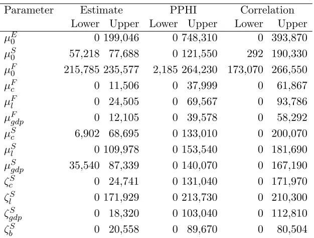
We estimate our model for the manufacturing sector of chemicals and chemical products (sector 24 according to 2-digit ISIC rev.3.1). The results show that standard gravity variables have a significant effect on trade costs. The startup costs for a Chilean firm entering a country that is in South America, in which Spanish is predominantly spoken and that has similar GDP
per capita to Chile (e.g. Colombia) are estimated to be between 277,303 USD and 313,216
USD.1 These costs increase significantly when the destination country is not located in South
America (e.g. the entering costs for Spain are estimated to be between 347,549 USD and
429,675 USD). The increase coming from the destination country not having Spanish as
official language is smaller (e.g. the estimated interval for Brazil is 283,323 USD to 421,640 USD). Finally, when a country differs from Chile in all three gravity variables included in the
model, the estimated interval increases further and becomes 387,527 USD to 538,986 USD.
Concerning the extended gravity variables, language is the only one which is estimated to significantly reduce the cost of accessing a new country: previously serving a market that has the same official language as the destination country reduces country-specific entry costs between 19 and 28 percent.
The spatial dependence in export entry and exit generated by extended gravity effects has important implications for the interpretation of the gravity equation parameters as well as for trade policy.
Since Tinbergen (1962) pioneered the use of gravity equations to study bilateral trade flows, his specification has been widely used. A defining characteristic of the gravity equation introduced by Tinbergen (1962) is that trade flows between two countries are predicted to depend exclusively on some index of their economic size and measures of trade resistance between them. Anderson and van Wincoop (2003) were the first to take into account the effect of third countries and introduce a multilateral resistance term in the specification of an otherwise standard gravity equation. In their model, for a given bilateral barrier between two countries j and j′, higher geographical barriers between j′ and other countries will raise
imports from j. Extended gravity effects work in the opposite direction. Their existence
makes it beneficial for firms to direct their export activities towards “hub” markets that share characteristics with a large number of countries. This effect will increase exports to these countries not only from firms already exporting to connected countries but, in general, from every firm. Not controlling for this “hubness” variable is likely to result in an upward bias in the estimates of the effect of bilateral trade barriers.2
1
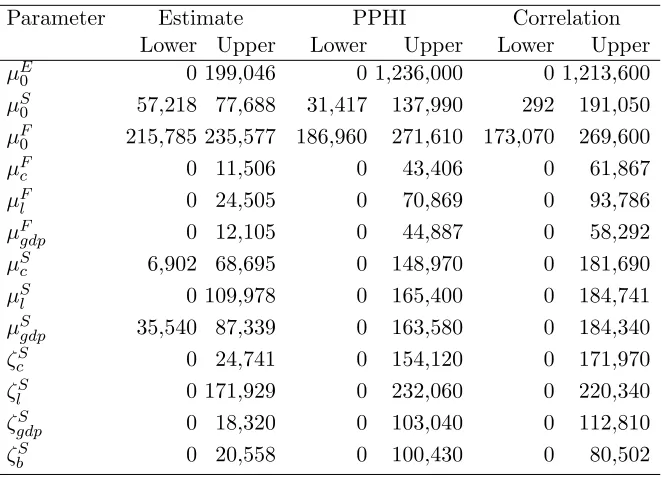
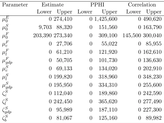
We report here the point estimates for the extrema of the identified set. Confidence intervals are provided in Section 8. Unless otherwise stated, every quantity included in this paper is evaluated in year 2000 US dollars.
2
Following the collapse of international trade that began in the last quarter of 2008, gravity equations have become a popular tool to estimate the elasticity of global trade with respect to
world GDP.3 Omitting the “hubness” variables makes these estimates particularly misleading.
Even under the assumption that the elasticity of bilateral trade with respect to the trade partner’s GDP is identical across any possible pair of countries, extended gravity effects imply that it is important to know how changes in global GDP are distributed across markets. A drop in GDP in a “hub” country, which is connected to many others through extended gravity, will have a much larger effect on aggregate trade than an equivalent change in a “non-hub” country that is isolated.
In addition to the consequences of extended gravity for the interpretation of parameters in gravity equations, the existence of extended gravity connections among the importing countries also has novel policy implications. Our model implies that reducing trade barriers in a country increases entry not only in its own market but also in other markets that are connected to it through extended gravity. This has important implications for import policies, suggesting that policies in one country will generate externalities for other countries. These externalities unveil a possible rationale for regional integration agreements, which force countries to internalize those cross-country effects when setting their legal barriers to trade. Concerning export policy, whenever there are reasons for export promotion measures, extended gravity points to the convenience of targeting these to hub countries that share characteristics with the largest number of foreign markets.
Our paper is related to several strands of the literature. First, our work relates to papers that structurally estimate fixed and sunk costs of exporting. Das et al. (2007), lacking data on export flows disaggregated by countries, estimate only general fixed and sunk costs of breaking into exporting. In contrast, we provide estimates in dollar values for country-specific fixed and sunk costs of exporting that vary depending on the characteristics of the destination country. Second, this paper also complements Albornoz et al. (2010), Chaney (2010), and Defever et al. (2010). The first two provide theoretical mechanisms that generate spatial patterns in sequential entry. Albornoz et al. (2010) assume firms have imperfect information about their export profitability, which they discover only after actually engaging in exporting. Assuming that profitability is correlated over time and across destinations, their model predicts that firms that have successfully entered some market are more likely to access countries that are similar to it. In contrast, Chaney (2010) builds a model in which exporters can break into a market only if they have a contact, and assumes that the probability of a given exporter acquiring such a contact in a new country is increasing in the aggregate trade flows between the
a given country are different for different countries of origin. Therefore, the standard practice in the gravity equation literature of introducing country-year dummies is not enough to control for the omitted “hubness” variable.
3
potential destination country and any other country that the exporter was previously serving. Furthermore, Albornoz et al. (2010) and Defever et al. (2010) present reduced form evidence showing that the geographical expansion paths that firms follow depend on their previous
destination markets.4 Our paper contributes to this literature by structurally estimating a
trade model that embeds a mechanism generating sequential entry.
Third, from a methodological point of view, our paper fits in the literature applying moment inequalities to the estimation of structural models. Like ours, many of these papers use this method as a way of handling choice sets that are large and complex (e.g. Katz (2007), Ishii (2008), Ho (2009)). The most closely related paper to ours is Holmes (2010), which studies Wal-Mart’s store location problem and quantifies the savings in distribution costs afforded by having a dense network. This paper’s moment inequality estimator relies on the assumption that Wal-Mart has perfect foresight and employs inequalities based on multiple-period deviations. In contrast, Pakes et al. (2006) and Pakes (forthcoming) discuss the possibility of applying an analogue of Euler’s perturbation method to the analysis of single agent dynamic discrete choice models without imposing perfect foresight. Our paper applies this approach. We allow agents to have expectational errors and show that only moment inequalities based on one-period deviations are compatible with consistent estimation in this setting.
The rest of the paper is structured as follows. In Section 2 we describe our data set, which we use in Section 3 to present reduced form evidence of the basic entry patterns we observe. Section 4 derives our model of firm entry into different export destinations, and Section 5 provides information on how we can derive moment inequalities from this model. Sections 6 and 7 describe the methods we use to estimate our parameters. Section 8 presents the baseline results, and Section 9 shows that they are robust to alternative specifications of the moment inequalities used in the estimation. Section 10 concludes.
2
Data Description
Our data come from two separate sources. The first is an extract of the Chilean customs database, which covers the universe of exports of Chilean firms from 1995 to 2005. The second
is the Chilean Annual Industrial Survey (Encuesta Nacional Industrial Anual, or ENIA), which
includes all manufacturing plants with at least 10 workers for the same years. We merge these two data sets using firm identifiers, allowing us to exploit information on the export
destinations of each firm and on their domestic activity.5
4
Albornoz et al. (2010) uses Argentinean data, and the results in Defever et al. (2010) refer to Chinese exporters. Although it is not the main focus of their paper, Eaton et al. (2008) shows additional evidence in the same direction for Colombian exporters.
5
These firms operate in the 19 different 2-digit ISIC sectors that deal with manufacturing.6 We restrict our analysis to one sector: the manufacture of chemicals and chemical products
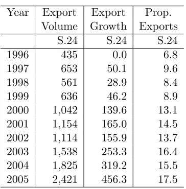
(sector 24). This is the second largest export manufacturing sector in Chile.7 As Table 1
shows, the volume of exports in the chemicals sector increased by approximately 19 percent on average during the sample period, and in 2005 it accounted for 17.5 percent of Chile’s manufacturing exports.
Our data set includes both exporters and non-exporters. Furthermore, in order to minimize the risk of selection bias in our estimates, we use an unbalanced panel that includes not only those firms that appear in ENIA in every year between 1995 and 2005 but also those that
were created or disappeared during this period.8
An observation in this data is a firm-country-year combination. For each observation we have information on the value of goods sold in US dollars. We obtain sales values in year 2000 terms using the US CPI. Basic summary statistics appear in Table 2. About 68 percent of our firms export at least one year of our sample period. These firms earn average revenues of over 1,390,000 USD per export market every year and have average domestic sales of 44,480,000 USD. In comparison, average domestic sales for nonexporters are 1,940,000 USD. Both distributions are nevertheless very skewed. The 75th percentile is in both cases significantly smaller than the corresponding mean. The average number of export destinations these firms serve per year is close to 6, and the median number is 4.
We complement our customs-ENIA data with a database of country characteristics. We obtain information on the primary official language and the names of bordering countries for
each destination market from CEPII.9 We collect data on real GDP, real GDP per capita,
and US dollar nominal exchange rates from the World Bank World Development Indicators. We use the Wholesale Price Index (or the Producer Price Index in those cases in which the Wholesale Price Index was not available) and nominal exchange rate data to build a bilateral real exchange rate index with respect to Chile. The source of the data on price indices is primarily the World Bank World Development Indicators, and the International Financial Statistics of the International Monetary Fund for those country-years for which the data was not available through the World Development Indicators.
have any exports listed with customs. In these cases, we assume that the customs database is more accurate in this respect and thus label these firms as non-exporters. We lose a number of small firms in the merging process because, as indicated in the main text, ENIA only covers plants with more than 10 workers. Nevertheless, the remaining firms account for around 80 percent of total export value.
6
ENIA encompasses class D (sectors 15 to 36) of the ISIC rev.3.1 industrial classification.
7
The largest export manufacturing sector is food and food products. The estimation results for this sector are still unavailable. They will be included in a new draft of this paper, which will be posted soon.
8
From our sample, we exclude only firms that appear in ENIA less than three years or that appear during two or more discontinuous periods between 1995 and 2005 (i.e. firms that first disappear and later reappear in the sample).
9Available at http://www.cepii.fr/anglaisgraph/bdd/distances.htm. Mayer and Zignago (2006) provide a
We construct our gravity and extended gravity variables from these country characteristics. The gravity measures compare Chile with each export destination. We create individual dummies that indicate if these export destinations share Chile’s language, continent, GDP per capita category, or borders. We use the World Bank classification of countries into GDP
per capita groups10. The extended gravity variables compare each country to a firm’s previous
export bundle. We have separate dummies for sharing language, continent, GDP per capita category, and border, with at least one country the firm exported to in the previous year, and not with Chile itself. More precisely, an extended gravity dummy (e.g. language) for a given firm-year pair and destination country takes on the value one if it does not share the corresponding characteristic with Chile (e.g. the destination country does not have Spanish as official language) but it does share this characteristic with some other country to which the firm was exporting in the previous year. As an example, Austria would take value of one for a given firm-year in all the four extended gravity variables if the firm exported to Germany in the previous period. We use dummy variables rather than continuous differences in order to simplify the interpretation of our strategy to build moment inequalities.
3
Preliminary Evidence
In this Section, we provide reduced form evidence that supports the choices made in the specification of the structural model.
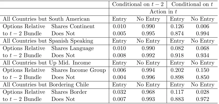
First, we consider why it is important to take into account extended gravity alongside the more conventional gravity forces. Table 3 presents transition matrices differentiating by extended gravity. The left panel of this table reports the probability that a firm entered a given country in a given year, conditioned on that firm-country-year observation falling into one of two groups. The first group contains those observations in which the firm was exporting in the previous period to a market that shares the corresponding characteristic (continent, language, GDP per capita group, or border) with the destination country. The second group includes those observations where the firm was exporting last period but not to any market that shares the same characteristic with this country. The right hand side of this table reports the probability that an observation falls into each of these two groups, conditioned on whether
or not it entered that country during the given period11.
10
The World Bank classifies countries into four groups (low, lower middle, upper middle and high income) based on their GDP per capita. The World Bank built these classifications using 2002 income per capita. Low income is 735 USD or less, lower middle income is 736 USD to 2,935 USD, upper middle income is 2,936 USD to 9,075 USD and high income is 9,076 USD or more.
11
If our extended gravity story holds, we expect that membership in the first group, where the firm exports in the previous period to a destination that shares the corresponding char-acteristic, raises the probability of entry relative to the case where the firm does not export to such a destination. This prediction bears out in all the panels of Table 3, since the top left hand entry is always substantially larger than the entry directly below it. Observations in which the firm previously exported to a country that shares the corresponding characteristic also account for a significant portion of the entry events that appear in the data. They are clearly the majority in all panels except for border and language. This is not surprising given that most countries share borders and official languages with very few other countries.
Although we argue that these tables support the inclusion of extended gravity in our model, there are other possible explanations for these findings. For example, imagine a model where continents are ranked in terms of their proximity to Chile, and firms tend to spread out gradually to more distant continents (i.e. entry is purely determined by standard gravity factors). In this case, the fact that a firm is already exporting to a certain continent would increase the probability that they will soon export to more countries on that continent. But the relationship would be driven by the distance between Chile and that continent, not between countries in that continent. However, it is harder for such a story to rationalize the language and border matrices. The model would have to predict that languages can be ranked by complexity in such a way that firms would access countries whose official language is up in the scale only when they have previously accessed the countries with “easier” languages. In the same way, the border variable in the model would have to generate a pattern where firms spread outwards from Chile through countries that physically touch each other. Yet, that conjecture then generates an extended gravity relationship, since it depends on borders between countries that do not include Chile. This analysis shows how important it is to control for gravity factors in order to correctly identify extended gravity effects. Our structural model takes this identification issue into account.
In the structural model we develop in the next sections, we assume that the state vector of a firm is defined based only on its export status in the previous period. This assumption implies: (1) extended gravity effects last only for one period; (2) every firm that did not export to a country in a given period has to pay full entry costs if it exports to it in the next period; (3) every firm that did not export at all in a given period has to pay the full basic costs of reentering into the export activity if it exports to any country in the next period.
Table 4 shows that the intensity of the extended gravity effects decreases very fast between lags one and two. In particular, the probability of entering a country in periodtgiven that the firm was exporting to some other country that shares a characteristic with it is, on average,
divided by 3 when that export event happened int−2 instead oft−1. In the same way, the
probability of exporting to a country in periodtgiven that the firm was exporting to the same
to this country int−2 and not int−1. Finally, the probability of exporting to some country
in t for exporters in period t−1 is 0.9065 and it decreases to 0.3472 when we condition on
exporting int−2 and not in periodt−1. Therefore, in an extension of the finding in Roberts
and Tybout (1997), not only does the general export persistence decay very fast, but the same can be said for persistence of exporting to a given country and extended gravity effects.
4
An Empirical Model of Export Entry
In this section, we present a partial equilibrium model where producers based in Chile and operating in a particular sector choose in every period the set of foreign countries they want to serve, in order to maximize their expected flow of profits. We take the creation and destruction of firms as exogenous and endogenize their supply decision in each foreign market. The following model is assumed to apply to any sector and, in particular, to the sector of chemicals and chemical products considered in the empirical section.
Sections 4.1 and 4.2 describe, respectively, the demand and the supply sides of the model. Given the setting introduced in these two sections, subsection 4.3 then shows how to derive constraints on the observed behavior of firms that can be used for estimation and inference. These constraints are defined through moment inequalities. Specifically, subsection 4.3 de-scribes a general method to derive moment inequalities in a dynamic discrete choice setting in which perfect foresight on the part of the agents is not necessarily imposed.
4.1 Demand
Each country j is populated by a representative consumer who has a constant elasticity of
substitution (CES) utility function over the different varietiesiavailable in each sector:
Qjt =h
Z
i∈Ajt
q
η−1
η
ijt di
i η
η−1
, η >1
where Ajt represents the set of available varieties, η is the elasticity of substitution between
varieties in the sector, andqijtis the consumption of varietyi. Given this utility function, the resulting demand for each variety is:
qijt = p
−η ijt
Pjt1−ηCjt (1)
whereCjt is the total consumption of countryjin the sector to which varietyibelongs,12and
Pjt is the sectoral price index in countryj:
12
Pjt =h
Z
i∈Ajt
p1ijt−ηdii
1 1−η
4.2 Supply
Each variety is produced monopolistically by a single-product firm. We identify each firm by
the same subindexithat identifies varieties. These firms are located in Chile but may sell in
every countryj. A firm serving marketj may face four different types of costs:
(1) marginal cost or cost per unit of output shipped to market j. It includes production
costs, transport costs, taxes and tariffs. It is denoted asmcijtand assumed to be constant.13
We model the marginal cost that firmifaces in country j at periodt(in logs) as:
ln(mcijt) = ln(fit) + ln(gMjt) +ǫMijt
wherefitdenotes the effect of firm characteristics,gM
jt captures the effect of destination country
characteristics, andǫMijt is an error term. We assume the following functional form forfit:
ln(fit) =β0M +βdsMln(domsalesit) +βsMskillit+βwMln(avgwageit) +βvaMln(avgvaladdit)
whereβM
0 is a constant, domsalesis sales revenue in Chile, skill indicates the proportion of
skilled workers, avgwageis the average wage in the firm, and avgvaladddenotes the average
value added per worker. The four variables are used as proxies for the firm’s unit cost function.
Concerning the term gM
jt we impose:
ln(gMjt) =βtM+βarMavlrerj+βdrMdvlrerjt+βlMlawj+βbMborderj+βcMcontj+βMl lanj+βgpcM gdppcj
whereβM
t is a time effect,avlrer and dvlrer capture, respectively, the sample mean and the
corresponding year-to-year deviations of the real exchange rate (in logs), lawis a measure of
the quality of legal framework, andborder,cont, lan, and gdppc are dummies that indicate,
respectively, whether the destination country shares border, continent, official language, or GDP per capita classification with Chile. Most of these variables are standard in the gravity equation literature as proxies for international transport costs and, therefore, we refer to them asgravity variables. We allow the long term effect of the real exchange rate (captured by βM
ar)
to be different from the short run effect (βM
dr). The GDP per capita dummy is included as
proxy for within-country transport costs and quality of judicial institutions.
13
(2) fixed cost faced by the firm every year it is exporting to marketj, independently of the quantity exported and of its previous exporting history in this or in other foreign markets. It encompasses, among other factors, the cost of marketing campaigns, expenditures on updating information on the characteristics of the market, and the cost of participation in fairs. It is denoted as f cijt and modeled as:
f cijt=gjF +ǫFijt (2)
wheregjF is a term that depends on observable gravity variables andǫFijtis an error term. The termgF
j is modeled as:
gjF =µF0 +µFc contj+µFl lanj+µFgpcgdppcj (3)
wherecont,lan, and gdppc are the same dummy variables included in the expression forgM
jt.
(3) sunk cost or startup cost faced by firms that were not exporting to country j in the
previous period. These sunk costs account, among other factors, for the costs of building distribution networks, hiring workers with specific skills (e.g. knowledge of foreign languages), and acquiring information about country-specific preferences and legal requirements needed to commercialize products in that country. We account in the model for the possibility that these costs are smaller for those firms that have been previously exporting to countries similar toj. The intuition is that these firms might have already gone through a big part of the adaptation
process that generates these sunk costs before actually accessing country j. Therefore, we
introduce a term that accounts for the effect of the previous exporting history of the firm on sunk costs:
scijbt−1t=g
S
j −eSjbt−1 +ǫ
S ijt
wheregS
j depends on observable gravity variables,eSjbt−1 depends onextended gravityvariables,
and ǫSijt is an error term. Theextended gravity term captures the reduction in the sunk cost
of exporting to countryj for a firm that in the previous period was exporting to the bundle
of countriesbt−1.14
The gravity term in sunk costs is modeled analogously to the one in fixed costs:
gSj =µS0 +µSccontj+µSllanj +µSgpcgdppcj (4)
while the extended gravity term is specified as:
ejbSt−1 =ζbSborderjbet−1 +ζcScontejbt−1+ζlSlanejbt−1 +ζgdpS gdppcejbt−1 (5)
wherebordere,conte,lane, andgdppce are dummy variables that take value one if the bundle
14
of countriesbt−1 to which the firm was exporting in the previous period includes at least one
country that shares, respectively, border, continent, official language, and GDP per capita
group with the destination country j and that characteristic is not shared by the country of
origin of the firm (i.e. Chile).15
Note that the extended gravity termeS
jbt−1 will be zero when: (a) firmidid not export in
the previous period; (b) firmiexported only to countries that do not share border, continent,
official language, nor GDP per capita group with countryj; (c) countryj shares border with
Chile, is in South America, has Spanish as official language, and is classified as an Upper Middle Income country.
(4) basic cost or startup cost that the firm must pay if it was not exporting to any country in the previous period. This fourth type of trade cost is included in the model in order to account for the bureaucratic costs in permits and licenses that a firm must face when starting to export. Note that it is paid only once, no matter to how many countries the firm is starting to export in period t. It is denoted bybc and it is modeled as:
bcit=µB0 +ǫBit (6)
whereµB0 is a constant, and ǫBijt collects the unobservable factors.
The model described above includes 36 parameters: 23 of them enter the expression for the
gross profits from exporting, including 11 time effects (β); 4 enter the expression for fixed
costs (µF); 8 appear in the expression for sunk costs (µS, ζS); and 1 in the basic costs (µB).
We group all these parameters into a single parameter vectorθ= (β,µF,µS,µB,ζS). Section
6 specifies all the assumptions on the statistical properties of the error terms (ǫM
ijt, ǫFijt, ǫSijt, ǫB
it).
4.3 Firm’s Optimization Problem
We use the structure described above to derive moment inequalities. These inequalities arise from firms’ optimizing behavior. We can split the optimization problem faced by firms in
every period into two sequential problems: (a) first, firms solve a static optimization
prob-lem and choose an optimal price and quantity in every country conditional on serving that
country; (b) second, firms solve a dynamic optimization problem and choose the bundle of countries to which they will supply a positive amount of output. Subsection 4.3.1 describes the static problem and subsection 4.3.2 analyses the dynamic one. Subsection 4.3.3 maps firms’ optimizing behavior into moment inequalities.
15E.g. the extended gravity variable
lanetakes value 1 if countryjshares official language with at least one country included in the bundle of countriesbt−1 and that language is not the official language of Chile (i.e.
4.3.1 Static Problem of the Firm
We begin by deriving the maximum gross profits that a firm may earn in a countryj
condi-tional on operating in it. These are defined as revenue from exporting minus variable trade costs. Given the assumption of constant marginal trade costs, the variable trade costs are just
the product of these marginal costs and the quantity exported. Therefore, the gross profits
are defined as profits before accounting for fixed, sunk, or basic costs.
A continuum of varieties is supplied in every country. Therefore, each supplier sets its
price in country j taking the sectoral price index, Pjt, as given. Taking into account our
demand structure, this means that firms set a fixed multiplicative markup over marginal cost. As a result, the price in marketj is:
pijt= η
η−1mcijt
Plugging this price into our demand (see eq.(1)) gives the revenue earned by firmiin country
j:
rijt= η
η−1
mcijt Pjt
1−η
Cjt (7)
Fixed markups and constant marginal costs imply that the maximum gross profits for firm i
of exporting to countryj at periodt are proportional to revenue:
vijt= 1
ηrijt (8)
4.3.2 Dynamic Problem of the Firm
As indicated above, in addition to marginal costs, firms may have to pay fixed, sunk, and
basic costs when exporting to a set of countries bt. We define net profits from exporting as
export profits after accounting for all the possible trade costs. Specifically, we can write the net profits for firmiof exporting to countryjat periodtgiven that it exported in the previous period to a bundle of countriesbt−1 as:
πijbt−1t=vijt−f cijt−✶{j /∈bt−1}scijbt−1t
where ✶{j /∈ bt−1} is an indicator function for firm i not exporting to country j in t−1.
Aggregating across countries we obtain the total net profits for the current export bundlebt:
πibtbt−1t=
X
j∈bt
πijbt−1t−✶{bt−1=∅}bcit
where✶{bt−1=∅} is an indicator function for firminot exporting at all in t−1.
use ot to identify the observed export bundle in that period t (i.e. the bundle selected by
a firm in t). Assumption 1 below indicates how the choice of this bundle is made. While
Assumption 1 is compatible with firms being perfectly forward looking and taking in every period the export decision that maximizes the expected value of the sum of discounted profits over an unbounded horizon, it is weaker than this and allows for other decision criteria that firms might have.
Assumption 1 Let us denote by oT
1 ={o1, o2, . . . , oT}the observed sequence of bundles
cho-sen by any given firmibetween periods1andT. Given a sequence of information sets for firm
iat different time periods, {Jit,Jit+1, . . .}, a sequence of choice sets from which firmipicks
its preferred export bundle, {Bibt−1t, Bibtt+1, . . .}, and a particular conditional expectation
functionEi[·]capturing its subjective expectations:
ot= argmax
bt∈Biot−1t
Ei
Πibtot−1t|Jit
∀ t= 1,2, . . . , T (9)
where
Πibtot−1t=πibtot−1t+δπibt+1btt+1+ωibt+1t+2,
the term ωibt+1t+2 is any arbitrary function of the discount factor, δ, and the static export
profits the firm might obtain in periods t+ 2and after:
ωibt+1t+2 =ωit+2(δ, πibt+2bt+1t+2, πibt+3bt+2t+3, . . .),
and the bundle bt+s is defined as the optimal bundle that would be chosen at period t+s if
the bundlebt+s−1 was chosen at period t+s−1:
bt+s = argmax
bt+s∈Bibt+s−1t+s
Ei
Πibt+sbt+s−1t+s|Jit+s
, ∀s≥1.
Assumption 1 links the observed export choices made by each firm in each period with the
structure described in sections 4.1 and 4.2. It models firm’s choice at periodtas the outcome
of an optimization problem that is defined by four elements: (1) a function Πibtot−1t; (2) subjective expectations, as captured by a conditional expectation function,Ei[·]; (3) knowledge
about the relevant environment included in an information set,Jit; and, (4) the set of options
taken into account by the firm (i.e. possible combinations of foreign countries to which firmi
considers exporting), as defined by a choice or consideration set,Biot−1t.
16
16
Note that we allow the consideration set of firmiat periodtto depend on the bundle of countries it chose in the previous period. Also note that the bundles{bt+s}s≥1 are random variables from the perspective of
periodt. The reason is that the value of{bt+s}s≥1depends on the information sets{Jt+s}s≥1, and these one
Assumption 1 does not impose any restriction on subjective expectations, information sets and consideration sets.17 However, it assumes that the function Πibtot−1t, which firms care
about when selecting the set of countries to which they export at period t, is a discounted
sum of the net profits obtained at t, πibtot−1t, the profits the firm will obtain at t+ 1 given the choicebtmade att,πibt+1btt+1, and an arbitrary function that is allowed to change across
firms, time periods and bundles chosen at t+ 1, ωibt+1t+2. Assumption 1 restricts ωibt+1t+2
to be a function of the discount factor and the static profits that the firm might obtain in periodst+ 2 and later.18
The introduction of the functionωibt+1t+2 makes the optimization defined in equation (9)
compatible with firms being forward-looking in many different degrees. Specifically, Assump-tion 1 is compatible with firms that take into account the effect of their current choices on future profits in any of the three following ways:
1. only one period ahead:
ωibt+1t+2= 0;
2. any finite numberp of periods ahead:
ωibt+1t+2=δ2πibt+2bt+1t+2+δ3πibt+3bt+2t+3+· · ·+δpπibt+pbt+p−1t+p
with
bt+s = argmax
bt+s∈Bibt+s−1t+s
Ei
Πibt+sbt+s−1t+s|Jit+s
∀s= 2, . . . , p;
3. or an infinite number of future periods ahead (i.e. perfectly forward looking firms):
ωibt+1t+2=Ei
Πibt+2bt+1t|Jit+2
with
bt+2 = argmax
bt+2∈Bibt+1t+2
Ei
Πibt+2bt+1t+2|Jit+2
.
In summary, Assumption 1 imposes only three constraints on firms’ behavior: (1) firms take into account the effect of their current choice on static profitsat least one period ahead;
17Propositon 1 and Assumption 2 impose some restrictions on these three elements. For details, refer to
the discussion contained in Section 4.3.3. Note in particular that Assumptions 1 and 2, and Propositon 1, are consistent with firms having rational expectations.
18
This characterization of the functionωibt+1t+2is more restrictive than necessary for our estimation method
to provide consistent estimates. In order for our moment inequalities to be correctly defined, the function
ωibt+1t+2may take any shape as long as it does not depend directly on the set of countriesbtselected att. Given
that any firmiexporting to any given bundlebt+s, for anys, will pay or not sunk and basic costs of exporting
depending only on the export bundle bt+s−1 (i.e. independently of bt+s−2, bt+s−3, . . .), the independence
betweenωibt
+1t+2andbt, conditional onbt+1, is guaranteed as long asωibt+1t+2is just a function of the discount
(2) firms internalize int that the set of countries to which they are going to export to in the
next period, bt+1, is a random variable and that it will be determined in t+ 1 by solving
an optimization problem analogous to the one they are facing in the current period; (3) the current choicebtenters the objective function of the firm only through its effect on the static profits in periodst andt+ 1, and on the choice bt+1 to be taken in period t+ 1.
4.3.3 Deriving Moment Inequalities: One-period Deviations
We apply an analogue of Euler’s perturbation method to derive moment inequalities. The the-oretical possibility of deriving moment inequalities by applying Euler’s perturbation method to the analysis of single agent dynamic discrete choice problems appears in Pakes et al. (2006) and Pakes (forthcoming). In adapting the intuition contained in these papers to our setting, we will form inequalities by comparing the actual sequence of bundles observed for a given firm
iwith alternative sequences that differ from it only in one period. Using the same notation
as before, oT
1 = {o1, . . . , ot, ot+1. . . , oT} denotes the observed sequence of country bundles
selected by a particular firm. We define an alternative sequence of bundles that differs from
oT
1 at a particular periodt:
{o1, . . . ot−1, o′t, ot+1. . . , oT},
where o′
t denotes a counterfactual bundle for period t. Note that when the firm makes the
choice at period t the bundles of countries that will be chosen in future periods are random
variables,{ot+s}s≥1, as they depend on factors included in future information sets,{Jt+s}s≥1,
that might be unknown to the firm at periodt.
Proposition 1 If o′
t∈ Biot−1t and all the possible realizations of ot+1 are in Bio′tt+1, then:
Ei[πiotot−1t+δπiot+1ott+1|Jit]≥ Ei[πio′
tot−1t+δπiot+1o′tt+1|Jit], (10)
and
ot+1 = argmax
bt+1∈Biott+1
Ei
Πibt+1ott+1|Jit+1
.
The proof of Proposition 1 is contained in Section A.1 in the Appendix.19 Intuitively, if the
bundle that would be chosen at periodt+ 1 conditional on choosingotat periodt,ot+1, could
have been chosen even ifo′
thad been picked (instead ofot), then the sequence{o′t,o′t+1}, where
o′
t+1 is the bundle of countries that the firm would have picked att+ 1 had the firm exported
too′
tin the previous period, is weakly preferredat periodtover the sequence{o′t,ot+1}. Since otwas preferred overo′
t, then transitivity of preferences insures that the export path{ot,ot+1}
was weakly preferredat periodt over the alternative path{o′
t,ot+1}.
19
Note that we use the boldfaceot+1to denote the random variable whose realization is the observed bundle
Equation (10) refers to the preferences of the firm at the time it had to choose between the actual and the counterfactual bundle and, therefore, it does not rule out the possibility that,ex post, the export path{o′
t, ot+1}could have generated higher profits than the observed
{ot, ot+1}.20 Assumption 2 below imposes a connection between the preferences of firms at
any time period and the actual realization of the differences in profits between two alternative export paths.
Proposition 1 imposes some constraints on the counterfactual bundles we can use to build
moment inequalities. It requires in particular that the counterfactual bundle, o′
t, belongs
to the consideration or choice set of the firm at period t, and that the firm could have still
chosen the bundle indicated byot+1even if it pickedo′tat periodt. As shown in Section 5, the
counterfactuals we use in the estimation diverge from the actual ones in that either they add or subtract one country to the bundle, they switch one export destination for an alternative one, or they exit exporting completely. Therefore we are implicitly assuming choice sets for
each firm and time period that includeat least the actual observed choice and a small number
of variations around it.21
In order to simplify notation, we rewrite the inequality in equation (10):
Ei[πidot+1t|Jit]≥0 (11)
whered= (ot, o′
t) denotes a particular deviation at period tand:
πidot+1t= (πiotot−1t−πio′
tot−1t) +δ(πiot+1ott+1−πiot+1o′
tt+1)
Given that the inequality in equation (11) holds for every possible deviationd, we can
aggre-gate across deviations in a single inequality. These deviations might differ in the alternative bundle of countries, o′
t, used to build the deviation d, in the firm, and in the time period in
which it is applied. We can therefore build a generic inequality as:
1
Dk I
X
i=1
T
X
t=1
Dk it
X
d=1
Ei[πidot+1t|Jit]≥0
20
More precisely, note that Proposition 1 does not imply:
Ei[πiotot−1t+δπiot+1ott+1|Jit]≥ Ei[πio′
tot−1t+δπiot+1o′tt+1|Jit],
nor
πiotot−1t+δπiot+1ott+1≥πio′tot−1t+δπiot+1o′tt+1,
whereot+1is the bundle to which firmiis observed to export at periodt+ 1. 21
and Dk=PI
i=1
PT
t=1Dkit is the number of observations used in the inequality.22
Finally, in order to derive moment inequalities from these theoretical inequalities, we need to restrict the behavioral expectations of the agents. The following assumption imposes the necessary constraint on the set of conditional expectation functions {Ei[·]}Ii=1.
Assumption 2 There is a positive valued function gkl(·) and an xidt ∈ Jit such that:
1 Dk I X i=1 T X t=1 Dk it X d=1
Ei[πidot+1t|Jit]≥0 ⇒ E
h 1 Dk I X i=1 T X t=1 Dk it X d=1
πidot+1tgkl(xidt)
i
≥0, (12)
and E[·] denotes the statistical expectation or expectation with respect to the data generation process.
Intuitively, Assumption 2 implies that agents make the right choices on average, where the average is computed across choices made by different firms in multiple periods and with respect to multiple alternatives or counterfactuals. Aggregating across firms, years, and deviations has the advantage of making Assumption 2 robust against expectational errors that are correlated across firms in a single year, or across firms and years in a single country. Assumption 2 does not impose that every firm must have rational expectations (i.e. Ei[·] = E[·], ∀i) but it is
consistent with it. In the same way, Assumption 2 is not violated either if firms are assumed to have perfect foresight.
Assumption 2 does not specify the information set of the agents, Jit, but it imposes mild
restrictions on it. Specifically, it assumes that the variables used as instruments in the moment inequalities, gkl(xidt), are contained in the information set of the agent at the time it took
the decision from which we are deviating in the counterfactual. As can be seen in Section 5, the only instruments we will use are indicator functions that classify firms and countries into groups according to their size. Therefore, the only assumptions imposed on the information set of the agents is that they know their own volume of domestic sales and the GDP of the countries included in their consideration or choice sets.
Assumptions 1 and 2 are not enough to rely on likelihood methods to identify the true
vector of parametersθ. In order to derive a likelihood function from the model described in
sections 4.1 and 4.2, we would need to specify the function ωibt+1t+2 for every i and t, the expectation function Ei[·] for every i, the information set Jit corresponding to every i and t, and the specific choice set Bibt−1t that each firm considers in each period.
23 All these are
22Abusing notation, we use
Dk below to denote both the set of deviations used to build the corresponding
inequality and its cardinality.
23Specifically, Assumption 1 and 2 are compatible with (but not restrictive to) firms that: (1) are perfectly
elements on which we actually have very little information. In contrast, Assumptions 1 and 2
are enough to derive moment inequalities that allow us to identify the parameter θ.
5
Specifying Moments: Bounding Cost Parameters
As it will be shown in Section 6, we use moment inequalities to estimate the parameters
affecting fixed, sunk and basic costs24. For each of these parameters we build sets of moment
inequalities aimed at identifying both an upper and a lower bound. Building moments implies two steps: first, we identify all the possible observations that might provide information on
the lower or upper bound for each parameter (i.e. we find the setDk); second, we aggregate
those observations into one or multiple moments for each parameter-bound pair (i.e. we define different functionsgkl(·)). We illustrate here our procedure with two examples. Specifically, we
examine how we build moments to identify bounds for our baseline fixed cost parameter,µF
0,
and for the parameter that measures the extended gravity effect of language, ζS
l . Additional
examples are provided in the Appendix in Section A.2.
5.1 Identifying Observations
5.1.1 Example 1: Bounding µF
0
Imagine we observe a firm i with the following stream of gross profits in country j and an
associated export trajectory
Year 1 2 3 4 5
Profits vij1 vij2 vij3 vij4 vij5
Exports 0 1 1 0 0
where vijt denote the potential gross profits that firm iwould obtain in country j if it were
to export at periodt, 1 indicates that the firm is exporting toj and 0 indicates that the firm is not. A possible counterfactual would be
Year 1 2 3 4 5
Actual 0 1 1 0 0
Counterfactual 0 1 1 1 0
number of countries in the world). Given that the cardinality of this choice set is enormous and that computing the value function for each of its elements is unfeasible with currently available computational capabilities, a model that imposes these three restrictive assumptions cannot be estimated either through any method that relies on the specification of a likelihood function. Therefore, even if these three additional assumptions were imposed, we would still need to use moment inequalities to identify the different parameters of the model.
24There are a total of 13 parameters entering either fixed, sunk or basic costs: (
µF
0,µFc,µFl,µFgdp,µS0,µSc,
µS
where we delay the exit period by one year. Assume for simplicity that country j shares the same continent, language, and GDP per capita group with Chile, meaning that the gravity variables for these characteristics appearing in the fixed cost term take a value of 0. Then our counterfactual generates the following difference in profits
πido54 =−vij4+µ
F
0 +ǫFij4,
which generates an observation for moment inequality that identifies the lower bound forµF
0.
In order to get an observation that helps to identify the upper bound for µF0 we simply
flip the counterfactual and advance exit by one period,
Year 1 2 3 4 5
Actual 0 1 1 0 0
Counterfactual 0 1 0 0 0
This gives the difference in profits
πido43 =vij3−µ
F
0 −ǫFij3
Thus, we have an observation for the moment inequality that identifies the upper bound of
µF
0.
In most cases the parameter of interest will not be the only unknown to appear in an
observation. Following the previous example, if countryj had not been in the same continent
as Chile, the two observations described above would have been:
πido54 =−vij4+µ
F
0 +µFc +ǫFij4,
and
πido43 =vij3−µ
F
0 −µFc −ǫFij3
It is possible that parameters affecting fixed and sunk costs appear both in the same
inequality. Again modifying the original example, return to the case where country j is
assumed to share the same continent, language, and GDP per capita group with Chile (i.e. all the gravity and extended gravity variables entering fixed and sunk costs are going to take a
value of 0) and imagine that firmihad reentered countryj in period 5 in the actual strategy.
In this case the different in profits that contributes to identify the upper bound forµF
0 would
not be affected but the one that identifies the lower bound would now be:
πido54 =−vij4+µ
F
5.1.2 Example 2: Bounding ζS l
Imagine that the same firm i is exporting in year 7 to only one country. This country only
shares official language with some country j and it shares nothing with some other country
j′. The stream of profits and actual export strategies implemented in each countryj and j′
are:
Year 7 8 9
Countryj Profits vij7 vij8 vij9
Exports 0 1 0
Countryj′ Profits vij′7 vij′8 vij′9
Exports 0 0 0
A possible counterfactual would be:
Year 7 8 9
Actual Countryj 0 1 0
Countryj′ 0 0 0
Counterfactual Countryj 0 0 0
Countryj′ 0 1 0
where firmienters countryj′ instead of countryj. Assume for simplicity that countryj and
j′ take the same value of the standard gravity variables and that firm i does not export to
any country in year 9. Then our counterfactual generates the following difference in profits:
πido98 =vij8−vij′8+ζ
S
l −ǫFij8+ǫFij′8−ǫSij8+ǫSij′8 (13)
which generates an observation for the moment inequality identifying the lower bound forζS
l .
Once we impose that ζS
l must take a nonnegative value, this observation might be
uninfor-mative if firm iwould have preferred country j over country j′ even if the extended gravity
effect of language was zero.
As indicated above in the example forµF
0, other parameters will appear in this inequality
if, for example, countryjandj′ take different values of the gravity variables, firmiis observed
to continue exporting to countryj at period 9, etc.
If we are looking for an upper bound, then we need to find a year for which there was a
country that benefited from extended gravity effects in language in which firmidid not enter
and another country that did not benefit from these effects in which firmi actually entered.
By building a counterfactual that switches the export strategies in those two countries we find an observation that helps us identify the upper bound forζlS.
for language. We just need to find a pair of countries j and j′ that diverge in the particular
dimension we are interested in, and follow the same steps indicated above.
5.2 Aggregating Observations into Moments
Once we have searched over all firms, countries, and time periods in our sample for actual strategies and possible counterfactuals that help us identify the upper or lower bound for our parameters of interest, we need to decide how to aggregate those observations into inequalities. Assumption 2 imposes that each moment inequality should be an average across firms, years, and counterfactual countries but allows for some freedom in the deviations to include in each of the averages. With the aim of getting the tightest possible bounds, we work with four possible aggregation strategies (i.e. four possible moments) for each bound-parameter pair: (1) selection of firms (2) selection of countries; (3) no selection; (4) selection of firms and countries.
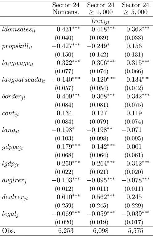
How do we select firms for cases (1) and (4)? We know from a regression of observed export revenue on exporter and destination country characteristics (see Table A.1) that higher domestic sales are correlated with higher predicted revenue from exporting in every country and time period. Therefore, as an example, when looking for a lower bound for the parameter
µF0, we obtain a higher lower bound if we build an inequality that averages only across the
observations coming from large firms (and the opposite for the case in which we are looking for an upper bound). We define firms as big if their domestic sales in the first year of the sample (i.e. 1995) were above the median (and vice versa). Given that larger firms have higher export profits in every country, the selection of firms is irrelevant in those moments
that compare profits between two countries (e.g. moments that identify bounds for ζS
l , see
Section 5.1.2).
How do we select countries for cases (2) and (4)? Table A.1 shows that higher GDP in the destination country is correlated with higher predicted revenue from exporting for every firm and time period. Therefore, keeping the same example as before, when looking for a lower
bound for parameterµF
0 we build an inequality that, for each firm, uses observations that come
from large countries (and the opposite when looking for an upper bound). When looking for
a lower bound for the parameter ζS
l we use counterfactuals that make the firm enter those
Not all these moments will be used in the estimation. Some of these aggregations for some of the bounds end up including very few observations. Even if Assumption 2 imposes only an asymptotic requirement on the moments used in the estimation, inequalities that use very few observations may have very large error components and can lead to very misleading results. We are explicit in Section 8 about the moments used to find our estimates.
Besides the different restrictions on the parameter space coming from the moment inequal-ities described above, we impose the following additional constraints on the possible values the parameters may take: (1) all the parameters must take non-negative values; (2) the parame-ters measuring extended gravity effects cannot take values such that the sunk cost of entering
some countryj for a firm exporting in the previous period to some other countryj′ becomes
negative. The difference between these constraints in the parameter space and those coming from moment inequalities is that the former are deterministic and, therefore, are imposed in every random sample.
6
Estimation Method
Once we have specified the different moment inequalities that identify the parameters entering the fixed, sunk, and basic costs, it remains to explain how these moments are going to be used to estimate those parameters. Section 6.1 lays out the linear moment inequality framework in general terms. Section 6.2 specifies how this framework maps to our setting and we explain in detail our estimation method.
6.1 The Linear Moment Inequality Framework
We focus here on identification and estimation of the extreme or boundary points of the identified set, while we leave for Section 7 the discussion about inference and how to build confidence intervals in the linear moment inequality framework. We follow the approach to estimation in models in which parameters are defined by moment inequalities contained in Pakes et al. (2006).
Let there be S linear moment inequalities, with each inequality indexed by s:
ms(θ) =Eh1
N N
X
i=n
(z0n+z1nθ+ǫn)g(z2n)
i
≥0 s= 1,2, . . . , S (14)
where N is the number of observations in the moment inequality,θis the parameter vector to
estimate, (z0,z1,z2) is a vector of observable variables, andǫ is an unobservable term. This
can be written as the set of valuesθ such that:
0 =
S
X
s=1
min{0, ms(θ)}2
We define an analog estimate ˆΘ of the identified set Θ as the set of values ofθ that minimize
the objective function:
S
X
s=1
min{0,ms˜ (θ)}2
(15)
where ˜ms(·) is the sample analog of the corresponding moment inequalityms(·)25:
˜
ms(θ) = 1
N N
X
i=n
(z0n+z1nθ)g(z2n)
As it is shown in Pakes et al. (2006), the bounds of ˆΘ are consistent estimates of the
corre-sponding bounds of Θ as long as the sample moments are uniformly consistent estimates of the population moments:
sup
θ
||ms˜ (θ)−ms(θ)||−−−−→N→∞ 0
Given the specification of the linear moment inequalities in equation (14), the uniform con-sistency of the sample moments is guaranteed as long as:
1
N N
X
n=1
ǫng(z2n) N→∞ −−−−→0
6.2 Mapping the Framework to our Model
As a result of Assumption 2, our model provides a set of S moment inequalities where each
moment inequalitysis indexed by the pair (k, l):
ms(θ) =Eh 1
Dk I X i=1 T X t=1 Dk it X d=1
πidot+1t(θ)gkl(xidt)
i
≥0 (17)
25
The objective function in equation (15) is a special case of more general Modified Method of Moments (MMM) test function defined in Andrews and Soares (2010):
S
X
s=1
`
min{0, 1 σs(θ)
ms(θ)}
´2
, (16)
whereσ2
s(θ) is the variance ofms(θ). Equations (15) and (16) are both going to generate the same identified
where θ = (β, µF, µS, µB, ζS) is the finite dimensional parameter vector that we want to
estimate.
The empirical model described in Section 4 parameterizes the difference in profits as:
πidot+1t(β, µF, µS, µB, ζS) =vidt(β)−gdF(µF)− gSdot+1(µ
S)−eS dot+1(ζ
S)
−bcdot+1(µB) +ε2d
where each of its terms is defined as:
vidt =
X
j∈ot
vijt−
X
j∈o′
t
vijt
gdF =X
j∈ot
gjF −
X
j∈o′
t
gjF
gSdot+1 =
X
j∈ot
✶{j /∈ot−1}gjS−
X
j∈o′
t
✶{j /∈ot−1}gjS
+δ X
j∈ot+1
✶{j /∈ot} −✶{j /∈o′t}
gSj
eSdot+1 =
X
j∈ot
✶{j /∈ot−1}eSjot−1 −
X
j∈o′
t
✶{j /∈ot−1}eSjot−1 +δ
X
j∈ot+1
✶{j /∈ot}eSjot
−✶{j /∈o′t}eSjo′
t
bcdot+1 =
✶{ot6=∅, ot−1 =∅} −✶{o′t6=∅, ot−1 =∅}
bc+δ✶{ot+1 6=∅, ot=∅} −✶{ot+16=∅, o′t=∅}
bc
ε2d=
X
j∈ot
ǫFijt−X
j∈o′
t
ǫFijt+ X
j∈ot
✶{j /∈ot−1}ǫSijt−
X
j∈o′
t
✶{j /∈ot−1}ǫSijt
+δ X
j∈ot+1
✶{j /∈ot}
−1{j /∈o′t}
ǫSijt+1+✶{ot6=∅, ot−1 =∅} −✶{o′t6=∅, ot−1 =∅}
ǫBijt
+δ✶{ot+16=∅, ot=∅} −✶{ot+1 6=∅, o′t=∅}
ǫBijt+1
and the definition of vijt, gFj ,gjS, eSjot−1, bc, ǫ
F
ijt, ǫSijt, and ǫBijt is given in equations (2), (3),
(4), (5), (6), and (8).
A comparison of equation (17) and equation (14) shows that our moment inequalities do not map exactly to the linear moment inequality framework described in Section 6.1 because
v(·) is a loglinear function of β. However, gF(·), gS(·), eS(·) and bc(·) are linear functions
of the corresponding parameter vectors. We will therefore estimate θ in two stages. In the
first stage, we apply linear panel data estimation techniques to obtain point estimates of β
that are independent of the value estimated for (µF,µS,µB,ζS). In the second stage, we use
the linear moment inequality framework in order to obtain set estimates for (µF,µS,µB,ζS)
6.2.1 First Stage Estimation
All the parameters entering the expression for the gross profits from exporting v(·) appear
also in the expression for the potential revenue from exportingr(·) (see equations (7) and (8)). Using data on observed export revenues for firms, countries and years with positive exports,
we obtain point estimates for the parameter vector β. In order to obtain these estimates in
the simplest possible way, we exploit the fact that the equilibrium equation for revenue from exporting that arises from solving the static problem of the firm is loglinear (see equation (7)).
Therefore we estimate β applying a fixed effects estimator on the equation:
ln(rijt) =βZijt+ (1−η)ǫMijt (18)
whereZijtincludes all the observable variables26appearing in equation (7) andǫM
ijtis assumed
to be independent ofZijt. Once we have obtained our estimates ˆβ, we define an approximation
to the potential gross profits from exporting for firmiin countryj at timetas:
ˆ
vijt=vijt( ˆβ) = 1
ηrijtˆ =
1
ηαˆexp( ˆβZijt)
where ˆα is defined as the OLS estimate of the only coefficient in a regression of rijt on
exp( ˆβZijt) that does not include a constant. The elasticity of substitutionη is not uniquely identified from the reduced form expression for export revenues. Therefore, we borrow the
value of η for from Broda et al. (2006)27. Given our approximation to gross profits ˆvijt we
define the first stage error as:
ε1ijt=vijt−ˆvijt
and
ε1d=
X
j∈ot
ǫ1ijt−
X
j∈o′
t
ǫ1ijt
6.2.2 Second Stage Estimation
Using the results from the first stage estimation, we can rewrite each of our moment inequalities as:
ms(θ2) =E
h 1 Dk I X i=1 T X t=1 Dk it X d=1 ˆ
vidt−gdF(µF)−gdSot+1(µ
S)+eS dot+1(ζ
S)−bc
dot+1(µB)+εd
gkl(xidt)
i
≥0
26We proxy the term
CjtPη−
1
jt with a power function of the GDP of countryjat periodt.
27