A Three-Stage Multiderivative Explicit
Runge-Kutta Method
Ashiribo Senapon Wusu1, Moses Adebowale Akanbi1*, Solomon Adebola Okunuga2 1Department of Mathematics, Lagos State University, Lagos, Nigeria
2Department of Mathematics, University of Lagos, Lagos, Nigeria Email: *[email protected]
Received January 10,2013; revised February 16, 2013; accepted March 18, 2013
Copyright © 2013 Ashiribo Senapon Wusu et al. This is an open access article distributed under the Creative Commons Attribution
License, which permits unrestricted use, distribution, and reproduction in any medium, provided the original work is properly cited.
ABSTRACT
In recent years, the derivation of Runge-Kutta methods with higher derivatives has been on the increase. In this paper, we present a new class of three stage Runge-Kutta method with first and second derivatives. The consistency and stabil- ity of the method is analyzed. Numerical examples with excellent results are shown to verify the accuracy of the pro- posed method compared with some existing methods.
Keywords: Multiderivative; Autonomous; Rung-Kutta; Stability; Convergence; Initial Value Problems
1. Introduction
The derivation of Runge-Kutta schemes involving higher derivatives is now on the increase. Traditionally, given an initial value problem (IVP), classical explicit Runge- Kutta methods are derived with the intention of perform- ing multiple evaluations of f y
in each internal stagefor a given accuracy. Recently, Akanbi [1,2] derived multi-derivative explicit Runge-Kutta method involving up to second derivative. Goeken and Johnson [3] also derived explicit Runge-Kutta schemes of stages up to four with the first derivative of f y
. However, thenew scheme is derived with the notion of incorporating higher order derivatives of f y
up to the second de-rivative. The cost of internal stage evaluations is reduced greatly and there is an appreciable improvement on the attainable order of accuracy of the method.
2. Derivation of the Proposed Scheme
The general form of a single step method for solving the Initial Value Problem (IVP)
, ,
0 0y x f x y y x y (1)
is defined as
1 , ;
n n T n n
y y h x y h (2)
where T
n, ;n
0
, ; ,
1 !
r r
T n n r
h
x y h f f x y
r x y
(3)and for the autonomous case of (1), in which y f y
,
, ;
T x y hn n
becomes
0
;
1 !
r r
T n r
h
y h f f y
r y
(4)The proposed scheme of this paper is of the form
1 3sMERK , ;
n n n n
y y h x y h (5)
where
3sMERK x y hn, ;n d k1 1 d k2 2 d k3 3
(6)
1 n
k f y
2 3 2
2 21 1 21 22
1 2
n y yy
k fy hb k c fh f c h f f ff
2 y
2
3 31 1 32 2 31
3 2 2
32 1 2
n y
yy y
k f y hb k hb k c fh f c h f f ff
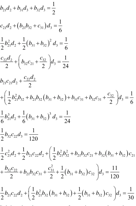
Expanding 2 and 3 in Taylor’s series and substi-
tuting the result into (5), the coefficients of the powers of are then compared with that of (3) to obtain the fol- lowing system of equations:
k k
h
x y h
is obtained using the Taylor’s se-
ries expansion of an arbitrary function:
1 2 3 1
d d d
21 2 31 3 32 3 1 2
b d b d b d
21 2 21 32 31 3 1 6
c d b b c d
22
21 2 31 32 3
1 1
2b d 2 b b d 1 6
32 22 2
32 21 3
1
2 2
c c d
b c d
24
22 2 21 21 2
2 32
21 32 21 32 31 32 31 31 32 31 3 2 1 1 6 2 2 c d b c d
c
b b b b b b b c b c d
33
21 2 31 32 3
1 1
6b d 6 b b d 1 24
32 22 3
1 1
2b c d 120
2 2 2
21 2 21 22 2 21 32 21 32 21 32 31 32 21 2
32 22 31
21 32 31 31 32 32 3
1 1 1
2 2 2
1 1
2 2 2 120
c d b c d b b b b c b b b c
b c c
b b c b b c d
1
221 22 2 21 32 31 32 31 32 32 3
1 1 1
2b c d 2b b b b 2 b b c d
1 30
Solving the above system of equations, we have the set of solutions in Table 1.
The above solution set gives rise to a family of 3-stage multi-derivative explicit Runge-Kutta schemes. The pro- posed scheme denoted by 3sMERK above is thus given by
1 1 2 4
6
n n
h
y y k k k3
2 3 2
2 1
2 1
5 10
n y yy
k fy hk h ff h f f ffy2
2 3 2
3 1 2
3 1 1 1
8 8 40 80
n y
2 yy
k f y hk hk h ff h f f ff
y 3. Convergence and Stability of the Method
3.1. Existence and Uniqueness of Solution
The properties of the incremental function
3sMERK x y hn, ;n
of the newly derived scheme are in
general, very crucial to its stability and convergence characteristics [1,4-8].
Theorem 3.1.
Let f x y
,
, where , be defined and continuous for all: n
f
n
x y, in the region defined by
a x b; y
, where a, b are finite, and let there exist a constant L such that
,
,ˆ ˆf x y f x y L yy (7) holds every
x y, , ,x yˆ D, then for any n,there exist a unique solution y x
of the problem (1), where y x
is continuous and differentiable for all
x y, D.The requirement (7) is known as the Lipschitz’s condi- tion, and the constant is a Lipschitz’s constants [6,
7,9-11]. We shall assume that the hypothesis of this theo- rem is satisfied by the IVP (1). The following lemma will be useful for establishing the aforementioned characteris- tics.
L
Lemma 3.2.
Let
i,i 0 1
n
be a set of real numbers. If there exist finite constants and such that
1 , 0 1 1
i i i n
, (8) then
0
1 , 1.
1
i
i i
(9)
Proof. Wheni0, (9) is satisfied identically as
0 0
.
Suppose (9) holds whenever i j so that
0 1 1 j j j
(10)
Then, from (8) i j implies that
1 .
j j
(11)
On substituting (10) into (11), we have
1 1 1 0 1 . 1 j j j
(12)
Hence, (9) holds for all i0. □
3.2. Accuracy and Stability
Usually, during the implementation of a computational scheme, errors are generated. The magnitude of the error determines how accurate and stable a scheme is. For instance, if the magnitude of the error is sufficiently small, the computational results would be accurate. However, if the magnitude of the error becomes so large, it can make the method unstable. The sources of error for these schemes and their principal error functions are discussed in Butcher [5,6], Fatunla [7] and Lambert [9, 10]. The following theorem guarantees the stability of the 3sMERK methods.
Theorem 3.3.
Suppose the IVP (1) satisfies the hypotheses of Theorem
.1, then the new 3sMERK algorithm is stable.
[image:2.595.58.286.85.430.2]Table 1. Examples of three-stage MERK methods.
Parameter Method1 Method2 Method3 3sMERK
1 d 169 816 1 6 1 9 1 9 2 d 5488
7089
1 16 636
1 16 6 36 1 6
3
d 125
6672
116 6
36
1 16 6 36 2 3 21 b 1728
16 6
10
16 6
10 1
31
b 91976
10625
3 402 197 6
1250 3 402 197 6
1250 3
8
32
b 108976
10625
2 489 179 6625
2 489 179 6 625 1 8
21
c 289
1568
37 2 6
100
37 2 6 100
2 5
22
c 17
196
154 19 6
500
154 19 6 500 1 5 31 c 3092 625
3 321 106 6
2500 3 321 106 6
2500 1
40
32
c 1823
625
342 37 6 2500
342 37 6 2500
1
40
Proof. Let n and n be two sets of solutions
generated recursively by the 3sMERK method with the initial condition
y z
0 0,
0 0, 0 0y x x z x z y z 0, and
,
n yn zn n
0
(13)
1 3sMERK , ;
n n n n
y y h x y h (14)
1 3sMERK , ;
n n n n
z z h x z h
(15)It implies that
1 1
3sMERK , ; 3sMERK , ;
n n
n n n n n n
y z
y z h x y h x z h
Applying triangle inequality and (13), we have
1 1 ,
n h n n
0
If we assume , and , then Lemma
3.2 implies that
1 h
0
0 n K
, where e b a
K
□ . This implies the stability of the 3sMERK scheme.
4. Numerical Experiments
The proposed 3sMERK scheme (6) is applied to the two IVPs below and the results obtained are compared with the standard 3-stage methods of Runge-Kutta (Heun’s)
[7,9,10] and that of Goeken and Johnson [3] stated in (16) and (17) respectively.
4.1. Heun’s Scheme
1 1 1 2 1 3 2 3 4 , , 3 2 . 3 n n n n n hy y K K
K f y
h
K f y K
h
K f y K
3 (16)
4.2. Goeken’s Scheme
1 1 2 3
1
2
2 1
3 1 2
4 , 6 , . 1 , 2 3 . 8 n n n
n y n
n
h
y y K K K
K f y
K f y hK h f y K
h
K f y K K
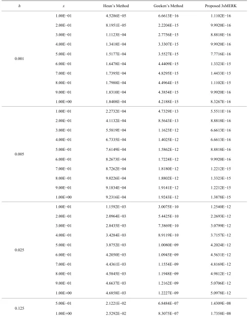
Table 2. The absolute values of error of y(x) in Problem 1 using the proposed scheme and other methods, h = 0.001; 0.005; 0.025; 0.125.
h x Heun’s Method Goeken’s Method Proposed 3sMERK
1.00E−01 4.5286E−05 6.6613E−16 1.1102E−16
2.00E−01 8.1951E−05 2.2204E−15 9.9920E−16
3.00E−01 1.1123E−04 2.7756E−15 8.8818E−16
4.00E−01 1.3418E−04 3.3307E−15 9.9920E−16
5.00E−01 1.5177E−04 3.5527E−15 7.7716E−16
6.00E−01 1.6478E−04 4.4409E−15 1.3323E−15
7.00E−01 1.7395E−04 4.8295E−15 1.4433E−15
8.00E−01 1.7988E−04 4.4964E−15 1.1102E−15
9.00E−01 1.8310E−04 4.3854E−15 9.9920E−16 0.001
1.00E+00 1.8408E−04 4.2188E−15 8.3267E−16
1.00E−01 2.2732E−04 4.7329E−13 5.5511E−16
2.00E−01 4.1132E−04 8.5643E−13 8.8818E−16
3.00E−01 5.5819E−04 1.1623E−12 6.6613E−16
4.00E−01 6.7335E−04 1.4025E−12 6.6613E−16
5.00E−01 7.6149E−04 1.5862E−12 8.8818E−16
6.00E−01 8.2673E−04 1.7224E−12 9.9920E−16
7.00E−01 8.7262E−04 1.8180E−12 1.2212E−15
8.00E−01 9.0226E−04 1.8802E−12 1.3323E−15
9.00E−01 9.1834E−04 1.9141E−12 1.2212E−15 0.005
1.00E+00 9.2316E−04 1.9243E−12 1.3878E−15
1.00E−01 1.1592E−03 3.0075E−10 1.2540E−12
2.00E−01 2.0964E−03 5.4425E−10 2.2693E−12
3.00E−01 2.8435E−03 7.3869E−10 3.0799E−12
4.00E−01 3.4284E−03 8.9119E−10 3.7157E−12
5.00E−01 3.8752E−03 1.0080E−09 4.2024E−12
6.00E−01 4.2050E−03 1.0945E−09 4.5631E−12
7.00E−01 4.4361E−03 1.1554E−09 4.8169E−12
8.00E−01 4.5845E−03 1.1948E−09 4.9812E−12
9.00E−01 4.6637E−03 1.2162E−09 5.0706E−12 0.025
1.00E+00 4.6858E−03 1.2227E−09 5.0978E−12
5.00E−01 2.1221E−02 6.8484E−07 1.4309E−08 0.125
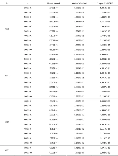
Table 3. The absolute values of error of y(x) in Problem 2 using the proposed scheme and other methods, h = 0.001; 0.005; 0.025; 0.125.
h x Heun’s Method Goeken’s Method Proposed 3sMERK
1.00E−01 6.0487E−07 8.8818E−16 8.8818E−16
2.00E−01 1.2336E−06 2.2204E−16 2.2204E−16
3.00E−01 1.8867E−06 4.4409E−16 4.4409E−16
4.00E−01 2.5647E−06 8.8818E−16 8.8818E−16
5.00E−01 3.2680E−06 1.3323E−15 1.3323E−15
6.00E−01 3.9972E−06 1.5543E−15 1.3323E−15
7.00E−01 4.7527E−06 1.5543E−15 1.3323E−15
8.00E−01 5.5351E−06 2.4425E−15 2.2204E−15
9.00E−01 6.3447E−06 1.5543E−15 1.3323E−15 0.001
1.00E+00 7.1821E−06 2.4425E−15 2.2204E−15
1.00E−01 3.0216E−06 4.4409E−16 0.0000E+00
2.00E−01 6.1625E−06 8.8818E−16 2.2204E−16
3.00E−01 9.4251E−06 1.5543E−15 4.4409E−16
4.00E−01 1.2812E−05 1.9984E−15 6.6613E−16
5.00E−01 1.6325E−05 2.2204E−15 8.8818E−16
6.00E−01 1.9968E−05 2.4425E−15 8.8818E−16
7.00E−01 2.3743E−05 2.6645E−15 6.6613E−16
8.00E−01 2.7651E−05 2.8866E−15 4.4409E−16
9.00E−01 3.1696E−05 3.1086E−15 2.2204E−16 0.005
1.00E+00 3.5879E−05 3.5527E−15 2.2204E−16
1.00E−01 1.5040E−05 1.9607E−13 0.0000E+00
2.00E−01 3.0674E−05 3.9857E−13 2.2204E−16
3.00E−01 4.6914E−05 6.0796E−13 4.4409E−16
4.00E−01 6.3773E−05 8.2401E−13 4.4409E−16
5.00E−01 8.1263E−05 1.0476E−12 4.4409E−16
6.00E−01 9.9397E−05 1.2779E−12 6.6613E−16
7.00E−01 1.1819E−04 1.5152E−12 6.6613E−16
8.00E−01 1.3764E−04 1.7601E−12 1.1102E−15
9.00E−01 1.5778E−04 2.0122E−12 1.1102E−15 0.025
1.00E+00 1.7860E−04 2.2717E−12 1.3323E−15
5.00E−01 3.9725E−04 6.4241E−10 1.4915E−12 0.125
1.00E+00 8.7330E−04 1.3932E−09 3.0043E−12
4.3. Problem 1
Consider the IVP
, 0 1
y y y (18)
with the theoretical solution e x
y .
4.4. Problem 2
Consider the IVP
2
, 0 1
4 80
y y
y y (19)
with the theoretical solution
4
20
1 19e
x
y
.
5. Conclusions
The results generated by the proposed scheme in this paper when applied to the problems above, evidently proved the extent of accuracy of the scheme. Tables 2
and 3 above show the absolute error associated with the
schemes for the test problems with the variation of the step length. The computations above clearly show the accuracy of the method. The standard Heun’s (third order) method grows faster in error than the method of Goeken and the newly derived scheme. However, 3sMERK per- formed best among the three methods.
Based on the two problems solved above, it follows that the scheme is quite efficient. We therefore conclude that the 3sMERK method proposed is reliable, stable and with high accuracy.
REFERENCES
[1] M. A. Akanbi and S. A. Okunuga, “On Region of Abso- lute Stability and Convergence of 3-Stage Multiderivative
Explicit Runge-Kutta Methods,” Journal of the Sciencea Research and Development Institute, Vol. 10, 2005-2006,
pp. 83-100.
[2] M. A. Akanbi, S. A. Okunuga and A. B. Sofoluwe, “Error Bounds for 2-Stage Multiderivative Explicit Runge-Kutta Methods,” Advances in Modelling and Analysis,Vol. 45, No. 2, 2008, pp. 57-72.
[3] D. Goeken and O. Johnson, “Fifth-Order Runge-Kutta with Higher Order Derivative Approximations,” Electronic Journal of Differential Equations,Vol. 2, 1999, pp. 1-9.
[4] M. A. Akanbi, “On 3-Stage Geometric Explicit Runge- Kutta Method for Singular Autonomous Initial Value Pro- blems in Ordinary Differential Equations,” Computing,
Vol. 92, No. 3, 2011, pp. 243-263.
doi:10.1007/s00607-010-0139-3
[5] J. C. Butcher, “Numerical Methods for Ordinary Differ- ential Equations in the 20th Century,” Journal of Com- putational and Applied Mathematics, Vol. 125, No. 1-2,
2000, pp. 1-29.doi:10.1016/S0377-0427(00)00455-6
[6] J. C. Butcher, “Numerical Methods for Ordinary Differ- ential Equations,” John Wiley & Sons Ltd., Chichester, 2003.doi:10.1002/0470868279
[7] S. O. Fatunla, “Numerical Methods for IVPs in ODEs,” Academic Press Inc., New York, 1988.
[8] A. S. Wusu, S. A. Okunuga and A. B. Sofoluwe, “A Third-Order Harmonic Explicit Runge-Kutta Method for Autonomous Initial Value Problems,” GlobalJournal of Pure & Applied Mathematics, Vol. 8, No. 4, 2012, pp.
441-451.
[9] J. D. Lambert, “Computational Methods in ODEs,” John Wiley & Sons, New York, 1973.
[10] J. D. Lambert, “Numerical Methods for Ordinary Differ- ential Systems: The Initial Value Problem,” John Wiley & Sons, London, 1991.