Estimation of Regression Model Using a Two Stage Nonparametric Approach

Estimation of Regression Model Using a Two Stage

Nonparametric Approach

Desale Habtzghi1, Jin-Hong Park2* 1_{Department of Statistics, University of Akron, Akron, USA} 2_{Department of Mathematics, College of Charleston, Charleston, USA}

Email: *_{[email protected],} *_{[email protected]}

Received April 2, 2013; revised May 2, 2013; accepted May 9, 2013

Copyright © 2013 Desale Habtzghi, Jin-Hong Park. This is an open access article distributed under the Creative Commons Attribu-tion License, which permits unrestricted use, distribuAttribu-tion, and reproducAttribu-tion in any medium, provided the original work is properly cited.

ABSTRACT

Based on the empirical or theoretical qualitative information about the relationship between response variable and co- variates, we propose a new approach to model polynomial regression using a shape restricted regression after estimating the direction by sufficient dimension reduction. The purpose of this paper is to illustrate that in the absence of prior in- formation other than the shape constraints, our approach provides a flexible fit to the data and improves regression pre- dictions. We use central subspace to estimate the directions and fit a final model by shape restricted regression, when the shape is known or is stipulated from empirical inspection. Comparisons with an alternative nonparametric regres- sion are included. Simulated and real data analyses are conducted to illustrate the performance of our approach.

Keywords: Dimension Reduction; Central Subspace; Polynomial Regression; Shape Restricted

1. Introduction

Even if the assumption of monotonicity, convexity or concavity is common, shape restricted regression has not been extensively applied in real applications for two main reasons. As the number of observations

 

n , the data dimensionality , and the number of constraints increases, computational and statistical difficulties (i.e. overfitting) are encountered, refer to [1,2] for de-

tailed discussion. These and other authors proposed dif- ferent methods to overcome the computational difficul- ties but there is no optimal solution.

 

d

 

m

To tackle these limitations, we estimate the direction by the sufficient dimension reduction and fit a final mo- del by the shape restricted regression based on the theo- retical shape or stipulated shape of the empirical results. The recent literature for the sufficient dimension reduc- tion proposed practical methods which provide adequate information about the regression with many predictors. Reference [3] considered a general method for estimating the direction in regressions that can be described fully by linear combinations of the predictors without assuming a model for the conditional distribution of Y X , where

and

Y X are response and explanatory variables,

respectively. They also introduced a method to estimate the direction in a single-index regression and [4] extend- ed it to multiple index regression by successive direction extraction.

More specifically, the main goal of this research is to show that the polynomial regression modeling by Central Subspace (CS) and Shape Restriction (SR) methods works well in practice, especially if the scatter plot shows a pattern. As is known that the curve fitting is finding a curve which matches a series of data points and possibly other constraints. This approach is commonly used by scientists and engineers to visualize and plot the curve that best describes the shape and behavior of their data. When more than two dimensions are used, we do not have the luxury of graphical representation any more but have theoretical information about the relationship of the response variable and predictors. Shape restricted regression is a non-parametric approach for building models whose fits are monotone, convex or concave in their covariates. Thses assumptions are commonly applied in biology [5], ranking [6], medicine [7], statistics [8] and psychology [9].

In general, one fits a straight line when the relationship between the response variable and the linear combination of the predictors is linear. Otherwise, one applies poly-

nomial, logarithmic or exponential regression to fit the data. These regressions are practical methodologies when the mean function with predictors is smooth. It is well- known that the estimation approaches from regression theory are useful in building linear or nonlinear relation- ships between the values of the predictors and the corre- sponding conditional mean of the response variable. See [10] for a detailed exposition of widely studied regres- sion methods, particularly polynomial regression. How- ever, the straightforward and efficient analysis may not be generally possible with many predictors. In many situ- ations when the underlying regression function or scatter plot has a particular shape or form, the fitted model can be characterized by certain order or shape restrictions. In this case, the shape restricted classes of regression func- tion are preferred. This nonparametric regression method provides a flexible fit to the data and improves regression predictions.

In addition, when the empirical results between the response and predictors appear to have a particular shape that has certain order or shape restrictions, the shape res- tricted regression functions may best explain the rela- tionships. Taking shape restrictions into account, one can reduce the model root mean square error or increase the power of the test. This improves the efficiency of a sta- tistical analysis, provided that the hypothesized shape restriction actually holds [11].

In order to contextualize the goal of this article, it is necessary to review the concept of CS and SR. In Section 2, we summarize the notion of CS and an estimation method of CS when the dimension is assumed to be known. Also, we suggest a data dependent approach to detect the unknown dimensions. In Section 3, we review the shape restricted regression and the constraint cone, over which we minimize the sum of squared errors of our approach for one dimension case. We apply our new approach to the simulated and a real data in Section 4. There are a few comments and concluding remarks in Section 5.

d

2. Estimation Method by Central Subspace

Let Y be a scalar response variable and X be a p1 covariate vector. Suppose the goal is to make an inference about how the conditional distribution Y X varies with the values of X. Then, the sufficient dim- ension reduction method is to find the number of linear combinations, T

1 , ,

Y X B XT , (1) where indicates independence, (1) holds when is a matrix whose columns form a basis for the subspace of . Therefore, a Dimension Reduction Subspace (DRS) for on

B

p 

Y X is defined as any subspace 

 

B of , for which (1) holds. Here is defined as the space spanned by the columns of . That is, (1) represents that Y is independent of

p

 

 

B

B

X given and

T

B X

1



p vector X can be replaced by the q1 vector . This indicates a useful reduction in the dimension of

T

B X

X , where all the information in X about is included in the -linear combinations. Here, (1) holds trivially for

Y q

p

I



B and a dimension re- duction subspace always exists. Hence, if the intersection of DRSs is itself a DRS, the Central Subspace (CS) is defined as the intersection of all DRSs, which is written as Y X

 

Bd for dimension d and Bd 



1, , d



.

That is, CS is the minimum DRS that preserves the original information relating to the data.

In this article, we use a method for estimating the CS,

 

d Y X B

 , which does not require a pre-specified model for Y X . If dimension d

 

p of CS are known, we need to estimate only the set of vectors



1, , d



. The

ultimate goal of this paper is to use these estimated vectors to fit a final model using SR, discussed in Section 3. While [12] considered multivariate kernel estimation of the predictor density, the method introduced in this paper uses one predictor at a time. As a result, it can reduce the computational complexity and avoid the spar- sity caused by high-dimensional kernel smoothing.

Suppose a matrix _ p q

h  with and define an information index

q p

 

 h by

 





 







 



T T

T

,

E log p Y E logp Y .

p Y p Y p

   

   

  

   

   

h X h X

h

h X (2)

The two forms in (2) are the informational correlation and the expected conditional log-likelihood, respectively. The idea behind this setting is to maximize the infor- mation index  over all p d matrices h when

T

I 

h h . Because p Y

 

does not involve , maxi- mizing

h

 

 h is equivalent to maximizing the expected conditional log-likelihood. This information index is similar to the Kullback-Leibler information between the joint density p



h XT ,Y



and the product of the mar-

ginal densities

 





 

h T p Y p

T

h X h X



, quantifying the depen- dence of on . The important properties of the above information index is supported by Pro- position 1 of [4].

Y

T

q

X   X

 , for such that the conditional distribution of

qp

Y X is the same as the conditional distribution of



T



1 T _{, ,}

q

Y  X   X . In other words, there would be no loss of information of pre- dictors if X were replaced by the linear com- binations. This is equivalent to finding a



matrix

q p



p q



₁, , _q





B   such that

 

_{ }



T

_

_T



_

1 , 1 log . n i i n

i _{i i}

p Y

n  p Y p

 h 



h X

h X

 

n

 h

w, ,

( 1 

is maximized over all matrices . Because the densities in n are practically un-

known, we use the nonparametric approach to estimate one-dimensional and multi-dimensional density estimates. Here, for the choice of kernels and selection of band- widths, we follow the general guideline proposed by [13]. Since the Gaussian kernel performed well for the simu- lated and real data sets, we use density estimates based on a Gaussian kernel for the one-dimensional density and a product of Gaussian kernels for the multi-dimensional densities. Let be the univariate Gaussian kernel,

be the vector, and 1 i be the observation. Then the -dimensional density estimate has the following form:

d p



a

h





T

i a



 h G T a w ) th i 1

a w , , w



1



1

1

1 1

, , a n a j ji ,

n a nj

i

j j nj

w w

p w w n b G

b           _ 









 

 _ (3)

where 1 4 a nj a j

b k s n  for j1, , a . s_j is the

corresponding sample standard deviation of wj and the constant ka









 

n  h T d 1 4

4 2 a

a 

  is the optimal bandwidth in the sense of minimizing the mean integrated square error from [13]. The density in is replaced by the estimates defined in (3) and maximize (4) for all

matrices such that d

p h h hI .

 





 





T T 1 , 1

ˆ n _log n i i

n

i _{n i n i}

p Y

n  p Y p

 h 



h X

h X (4) This method incorporates T _;

d I



h h it is the sequential quadratic programming procedure of [14].

Since prior information about d may not be avai-

lable in practice, it will be useful to find a simpler way to determine using the data. The sufficient dimension reduction methods have been proposed for the deter- mination of the minimal dimension of the CS. See [15-17] for details. In this paper, using the estimating function d



d



ˆ n

 h defined in (4), we suggest the follow- ing Akaike Information Criterion (AIC) to determine d.

 



,

ˆ ˆ

: arg min 2 n d p 2

d



AIC d  n h  dp (5)

3. Fitting Model with Shape Restricted

Regression

In this section, we review some fundamental concepts that can help us to lay the groundwork for the construc- tion of the shape restricted method. More details about the properties of the constraint cone and polar cones can be found in [11,18-21].

 

Y  f X 



T T



1 , , q _

X  X   X is model the errors i

where and :q .

f

In th  ’s are inde

st

pendent and have andard normal distributi . on f

 

 can be monotone,

convex or concave based on th alitative information about the relationship between response variable and predictors or empirical results.

For simplicity let q 1

e qu

 and i f x

 

i . n. The con 

 For q1

see [20,22] for detaile scussio straine over which we minimize the sum of squared errors is constructed as follows: the monotone nondecreasing constraints can be written as

1 2

d di d set

n

  

f

ine

The restriction of to the set o ex functions is ac

f conv complished by the qualities

3 2

2 1 1

2 1 3 2 1

. n n

n n

x x x x x x

  _            

In our case,

       i x e

is a realized value of the linear com- bination of th predictors; X is estimated using CS. Any of these sets of inequalities defines m half spaces

in n

R , and their intersection forms a closed polyhedral conv cone in n

R . The cone is designated by ex



: 0



 

C  A for m n constraint matrix A. Here, 1

m n

m n

fo 2

r monotone, nondecreasing con x and ve   for convex.

notone constraints, the nonzero elements of the For mo

n

m dimensional constraint matrix A are A_{i i,}  1 , 1 1

i i

A 

and  for 1  i n 1. For co ex co the nonzero element

nv nstraints s of A are A_{i i,} x_i₂x_i₁,

, 1 2

i i i i

A  xx and Ai i, 2 xi1 xi  

     . For e if n

for 1in 2 xample, 5, the monotone con traint matrix s A is given by

1 1 0 0 0 0 1 1 0 0 0 0 1 1 0 0 0 0 1 1

    _             A 5

n and the x

-If coordinates are equally spaced, the a

and

.

nondecreasing conc ve and convex constraints are given by the following constraint matrices, respectively:

1 2 1 0 0

 

 

0 1 2 1 0 , 0 0 1 2 1 0 0 0 1 1

 _{ }    _{ }        A

1 2 1 0 0 0 1 2 1 0 0 0 1 2 1

     _  _  _    A

Some computational details: The ordinary least- squares regression estimator is the projection of the data vector on to a lower-dimensional line r subspace of ontrast the shape restricted estimator can be y

. In c

a

n 

ob

xis

tained through the projection of y on to an m

dimensional polyhedral convex cone in n _{[23]. We}

have the following useful proposition which shows the e tence and uniqueness of the projection of the vector

y on a closed convex set (see [11]).

Proposition 1 Let C be a closed convex subset of

.

n



1) For _yn _and _{C, the following properties}

e equivalent: ar

a) yˆ minC y

b) y ˆ, ˆ 0 for all C 2) For every _yn

satisfies (a)

, there exists a unique point where ˆC an (b). d ˆ is said to be the pr

w e notation

ojectio ,

here th

n of y onto C

,b 



a_{i i}b

a refers to the vector

in and

sition

ner product of a b. It is easy to see that (1b)

of Propo 1 becomes

ˆ ˆ_{, 0 and}

 

y   y ˆ,

r

0, ,

   C (6)

which are the necessary and sufficient conditions fo  to minimize n₁





2

i i

y

i 



over

Let d by

for a monotone, nondecreasing convex,



and

C. nne

V be the linear space spa



1, ,1



T onde- 

1 and n creasing concave, and let V be the linear space spanned by 1



1,,1T 



x₁, , x_n



T for conve

re

x x

s. The con-gress . Note that VC in both case

straint cone can be specified by a set of linearly independent vectors 1_{, ,} m

ion

  s



: j1 j j 0



   



 and et as



: 1 : , , ,1 0 and



m j

j m j

jb b b b

 



  

C       V ,

wher

a

,

b b 

m j _{the constraint s}

e for monotone, nondecreasing concave, nondecreasi x and

vectors

1

m n

ng conve m n 2 for convex. The

j



, , m 

  

   C

can be the form

ple, any con obtained from

. For exam

ula vex





1 1_{ AA}  _A

vector  is a nonnegative linear combination of the j

 vectors plus a linear combination of 1 and x. If C is e set of all convex vectors in n, we can also de

th

fine the vectors  j _{to be the rows of the} following matrix:

3 2 1

2 2

0 0 0 1

0 0 0

n

n n

x x x x

                   2

4 3 1 3

3 3

1

0 0 0 0 0 1

n

n n

x x x x

x x x x

        _                     

For a large data set, it is better to use the above vectors

x x x x

  

j

 is com

because the previous method of obtaining the edges putationally intensive. Another advantage is that the computations of the inner products with the second approach are faster because of all the zero entries in the vectors.

The polar cone of the constraint cone is ([19], p. 121)







0   : ,   0,  .

 

Geometrically, the polar cone is the set of points in _n

which make an obtuse angle with all points in . Let us note some straightforward properties of 0:

1) 0 is a closed convex cone,

2) The only possible element in   0 is 0,

3) 1

0

, ,_ m_

   .

e

wher _j _{is negative rows of}

A, i.e., 1_{, ,} m _.

   A

   The following proposition is a useful tor

t

tool for finding the constrained least squares estima . Its proof was discussed in detail by [23].

Proposition 2 Given yn such tha

j j b j j j j b   





 



  , the projection of y onto the

J J

y

constraint set  is

ˆ j _. j j b   



 J

  (7)

and the residual vector ˆ ˆ j j jJ

b   y



   is the pro- jection of y onto the po e ₀.

If t e set

lar con J

h is deter constrained least squar

mined, using Proposition 2, the es estimate, ˆ, can be found through ordina leasry t-squares regression (OLS), using

V

 and j _for jJ

is fin the cone

as re It is clear that ber of iterations ite, a

of of . To find set gressors.

the the num

number

s there is only a finite and ˆ,

faces J

the mixed primal-dual b [18] or the hinge algo thm of [23] can be us . F

ases algo of

ri ed or monotone re-

gr o

t

upon r

nsion reduction for different sample sizes es context. They found t a true dimension is

rithm

ession the p oled adjacent violators algorithm, known as PAVA [11] may be used. A code of he algorithm was written in R. The code can be obtained from the authors

equest.

4. Numerical Illustration

We examined the performance of the proposed metho- dology using a real and four simulated data sets. For each of the simulated data set, we carried out the compu- tational algorithms as described in Sections 2 and 3 for sample size n = 100. Recently, [24] investigated a

sufficient dime

and dimensions in the time seri that the performance to detec

sets which have the worst scenario, n100 , and computationally less intensive dimensions, d1 and 2 only, to illustrate clearly how the shape restricted method works well in these directions. For the nonparametric alternative we used a kernel. Although optimal band- width selection is essential, we used data adaptive fixed bandwidth





 

0.2

max min 8

b x x n that was recom-

mended by [25]. Here xmax and xmin are the mum

and minimum values used in estimation, respectively, and n is the sample size.

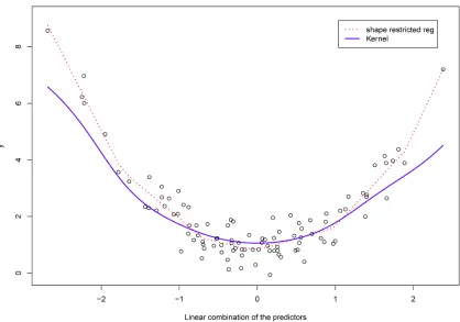
We considered quadratic regression model linear combination of six predictors for the first example and ten predictors for the second example. In the third example, we simulated data from cubic regression of a linear combination with ten predictors. The fourth ex-

ample is m mulated from two

dimensional model including ten dictors. In all the simulated data sets,

max

s of a i

ore complicated data si pre

 are independent standard normal random variables. Finally, we app proach to

lied our new ap a real data set, Highway Accident Data.

Example 1: Model 1









2

1 2 3 4 5 6

2 4 3 2 35 0.5 .

Y   x x  x  x x  x  

We simulated data from the above model where the mean fu unction of a linear combination with six predictors. First, we estimated the dimension and direction by CS combined with AIC (5) as described

nction is a quadratic f

in Section 2. As shown in Table 1, we detected a true dimension d1. We estimated a vector,





1

ˆ _{ 0.401,0.206, 0.668,0.525,0.130,0.241 ,}

 by the

algorithms described in Section 2. The scatter plot,

T 1

ˆ _X

 vs Y, shows a quadratic relation, see Figure 1. Then, based he scatter plot, we fitted t

convex regression was based on a visual examination of the

r plot.

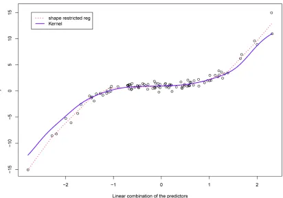
Example 2: Model 2

on t he data using

convex regression (SR). The decision to use the

scatte









2

1 2 4

1 2 2 6 0.5 .

Y    x x x   In this model, we cons

n of one linear com

idered another quadratic mean functio bination with ten predictors. Using the same procedures as the previous exa

estimated dimension and direction by CS. Based on AIC, mple, we

a true dimension d1 was detected, see Table 1 for details. The estimated vector is



0,0.003,0.013,0.013,0.046,0.029 .



1

ˆ _{ 0.815, 0.378, 0.004, 0.437,0  } 

The scatter plot of Figure 2, T 1 ˆ .00

















2

1 3 5 10

3

1 3 5 10

1 2 4

4 0.5

Y x x x x

x x x x

X

 vs Y , shows

.



    

    

quadratic relation. The scatter a rea- sonable choice of the relationship between the

plot suggested that

T 1

ˆ _X



nd is a convex curve. He model w

Y nce,

sho

we fitted a

a In this example, we simulated data from a cubic poly-

nomial model of one linear combination with ten pre- dictors. In the first step, we estimated dime nd direction by CS. Table 1 indicated that a true dimension

nsion a using convex regression. Figure 2 s that the shape

restricted regression fits the data better than kernel regression, which leads to a smaller error sum of squares.

Example 3: Model 3 d1 was detected by AIC. The estimated vector is



1

ˆ _{ 0.497,0.011,0.489,0.056,0.476,}

 0.019, 0.055, 0.071,0.030, 0.525  

_

.

The scatter plot, T 1

ˆ _X

 vs

we fitted a m the sh

ed e co ound

Y, sho of the inimi ncave-conve

w urve.

the second step,

ression based on ape scat ot. Our

estimator was comput by m of

uared errors over th n-

fl f m

ata. Exam s a cubic c

odel by concave-convex ter pl zing the sum

x set. The i

d See Figure 3 and Table 1 for details. ple 4: Model 4

In

reg

_

_









2 4 6 8

sq exp x₁ x₃ x₅ x₁₀ 4

4

0.1 ,

Y x x x x

    

w

    

ection point was by inimizing the sum of squared errors until the conditions in (6) were satisfied. Here, the shape restricted regression does fairly well in all ranges of the data set. The SR and kernel regression are almost on top of each other in the entire range of the

here d2 and p10. Here, we consider a non- ng two dimensions. Table 1 showe we estimated true dimensions

linear function incl d that

udi

2

d by

AIC. The two directions are



1

ˆ _{ 0.2468,0.4704,0.2715,0.4662,0.2357}

 and



ˆ _{ 0.3122, 0.2625,0.2117, 0.2094,0.389 }





,0.3895,0.0020,0.4492,0.0031,0.1330

0.1028, 0.1432, 0.1400,0.0

  



Figure 1. (Model 1) Data are generated from quadratic function of a linear combination with six predictors. The solid curve is quadratic fit and the dotted curve is the shape restricted fit.

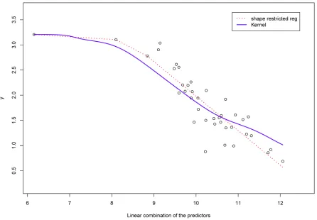
[image:6.595.90.515.83.378.2] [image:6.595.90.508.414.707.2]

[image:7.595.94.506.83.372.2]

Figure 3. (Model 3) Data are generated from cubic function of a linear combination with six predictors. The solid curve is cubic fit and the dotted curve is the shape restricted fit.

Table 1. AIC values for the simulated and a real data sets using Equations (5).

1 2 3 4





2

0

1 _ˆ ASEL N i i

i

Y Y N 







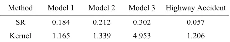
d _{The entries of the Table 2 are the square roots of the}

ASEL. The results from Table 2 demonstrate that our method performed fairly well in all cases. It is better than kernel regression, in particular, when the data is gene- rated from quadratic and cubic regressions. In general, we can see that our method provides better or compara- ble fits for the simulated examples, which is also sup- ported by the results of Figures 1-3.

Example 4: Highway Accident Data

For illustration, we applied our method to a real data set, Highway Accident Data. See Weisberg (2005) for a

detailed description about this data. The data include 39 sections of large highways in the state of Minnesota in 1973 and the variables relate the automobile accident rate in accidents per million vehicle miles to several potential terms. We use log(Rate) as a response variable and eleven

terms as explanatory variables. The definition of terms of this data is described in Table 10.5 of Weisberg (2005).

First, we estimated the direction of the predictor variables without losing any information using CS. As shown in Table 2, the dimension is detected by

Model 1 −78.94* _{−74.38 −61.78 −50.78}

Model 2 −79.78* _{−73.26 −61.10 −43.96}

Model 3 −42.78* _{−18.50 12.22 47.24}

Model 4 −116.46 −117.90* _{−97.88 71.96}

Highway Data −27.20* _{−26.08 −22.77 −11.31}

The response variable Y is non-decreasing in both predic-

tors



T T



1 2

ˆ _X, ˆ _X

  . In addition, the marginal scatter plots,

T 1

ˆ _X

 vs Y and ˆ₂TX vs display an increasing trends. Next, we fitted a model by a multiple isotonic re- gression. The isotonic fit is shown in Figure 4. This shows that our approach may be a better choice than parametric or nonparametric models that do not use the constraints and works well even for two dimensional model.

For the purpose of comparison, we computed Average Squared Error Loss (ASEL) of our models and alterna-

Y,

1

d

tive kernel regressions as the following: AIC. The estimated direction is

[image:7.595.55.287.438.551.2]

function which has two dimensional model including ten Figure 4. (Model 4) Data are generated from nonlinear m

predictors.

ean

Fig

[image:8.595.159.439.82.366.2] [image:8.595.76.522.409.719.2]

able 2. Average Squared Error Loss (ASEL) of the shape restricted regression and kernel regression.

Method Model 1 Model 2 Model 3 Highway Accident

T 371-384. doi:10.1093/biomet/92.2.371

[4] X. Yin, B. Li and R. D. Cook, “Successive Direction Ex- traction for Estimating the Central Subspace in a Multi- ple-Index Regression,” Journal of Multivariate Analysis, Vol. 99, No. 8, 2008, pp. 1733-1757.

doi:10.1016/j.jmva.2008.01.006

SR 0.184 0.212 0.302 0.057

Kernel 1.165 1.339 4.953 1.206

[5] G. Obozinski, G. Lanckriet, C. Grant, M. Jordan and W. Noble, “Consistent Probabilistic Outputs for Protein Func- tion Prediction,” Genome Biology, Vol. 9, No. 1, 2008, pp. 247-254. doi:10.1186/gb-2008-9-s1-s6

From the scatter plot of Figure 4, there is some curvature in the relationship between T

1

ˆ _X

 choice

vs . Hence, a con- cave curve may be a good to reflect the relation- ship between the response variable and the linear combi- nation of the predictors. Figure 4 shows the concave and cubic regression fits. The plot of Figure 5 and the ASEL in Table 2 suggests that our method gives reasonable fit to this data set.

5. Comments

The polynomial regression is one of handy methods in regression analysis. However, this straightforward analy- sis is not generally possible with many predictors. Hence, the major message that we would like to deliver in this paper is that the estimation of direction by CS and fitting the model by SR is advantageous for high dimensional data that has many predictors. After estimating the direc- tion by sufficient dimension reduction, it is not easy to choose the appropriate polynomial regression model from the pattern of the scatter plot without any theoreti-

al basi

h as bimodal

fu d c ve- . Fo c

the nform n is the

incr ng, c e, co b ) of the lying regression function, our approach provides m cept-

ble fits/estimates.

REFERENCES

sset and M. Shahar, “Decomposing Isoto- for Efficiently Solving Large Problems,”

Y

[6] Z. Zheng, H. Zha and G. Sun, “Query-Level Learning to Rank Using Isotonic Regression,” 46th Annual Allerton

Conference on Communication, Control, and Computing,

Allerton House, 24-26 September 2008, pp. 1108-1115. [7] M. J. Schell and B. Singh, “The Reduced Monotonic Re-

gression Method,” Journal of the American Statistical As-

sociation, Vol. 92, No. 437, 1997, pp. 128-35.

doi:10.1080/01621459.1997.10473609

[8] R. Barlow and H. Brunk, “The Isotonic Regression Prob- lem and Its Dual,” Journal of the American Statistical

Association, Vol. 49, No. 5, 1972, pp. 784-789.

[9] J. Kruskal, “Multidimensional Scaling by Optimizing Goodness of Fit to a Nonmetric Hypothesis,” Psycho-

metrika, Vol. 29, No. 1, 1964, pp. 1-27.

doi:10.1007/BF02289565

[10] S. Weisberg, “Applied Linear Regression,” Wiley, Ho- boken, 2005.

[11] T. Robertson, F. T. Wright and R. L. Dykstra, “Orde e- stricted Statistical Inference,” John Wiley & Sons, New r R c s. Furthermore, the parametric or nonparametric York, 1988.

models that do not use the constraints are not capable of

giving different shapes of actual fit suc [12] Y. Xia, “A Constructive Approach to the Estimation of Dimension Reduction Directions,” The Annals of Statis- tics, Vol. 35, No. 6, 2007, pp. 2654-2690.

doi:10.1214/009053607000000352

[13] D. W. Scott, “Multivariate Density Estimation: Theory, Practice, and Visualization,” John Wiley & Sons, New York, 1992. doi:10.1002/9780470316849

[14] P. Gill, W. Murray and M. H. Wright, “Practical Optimi- zation,” Academic Press, New York, 1981.

[15] K. C. Li, “On Principal Hessian Directions for Data Visu- alization and Dimension Reduc

nction an only avail

onca able i

convex atio

r such

shape (decreasing, onditions, when

easi oncav nvex or athtub under ore ac a

6. Acknowledgements

Jin-Hong Park is supported in part by the faculty research and development at the Mathematics Department and the College of Charleston.

tion: Another Application

of Statistics, Vol. 87, No. 420,

9.1994.10476455 of Stein’s Lemma,” Annals

1992, pp. 1025-1039.

[16] J. R. Schott, “Determining the Dimensionality in Sliced Inverse Regression,” Journal of the American Statistical

Association, Vol. 89, No. 425, 1994, pp. 141-148.

doi:10.1080/0162145 [1] R. Luss, S. Ro

nic Regression [17] Y. Xia, H. Tong, , “An Adaptive

Estimation of Roy-

W. K. Li and L. X. Zhu

Dimension Reduction,” Journal of the Proceedings of the Neural Information Processing Sys-

tems Conference, Vancouver, 6-9 December 2010, pp.

1513-1521.

[2] W. Maxwell and J. Muckstadt, “Establishing Consistent and Realistic Reorder Intervals in Production-Distribution Systems,” Operations Research, Vol. 33, No. 6, 1985, pp. 1316-1341. doi:10.1287/opre.33.6.1316

[3] X. Yin and R. D. Cook, “Direction Estimation in Single- Index Regressions,” Biometrika, Vol. 92, No. 2, 2005, pp.

al Statistical Society, Ser. B, Vol. 64, No. 3, 2002, pp.

363-410. doi:10.1111/1467-9868.03411

[18] D. A. S. Fraser and H. Massam, “A Mixed Primal-Dual Bases Algorithm for Regression under Inequality Con- straints. Application to Convex Regression,” Scandina-

vian Journal of Statistics, Vol. 16, 1989, pp. 65-74.

[image:9.595.57.288.113.156.2]

[20] E. Seijo and B. Sen, “Nonparametric Least Squares Esti- mation of a Multivariate Convex Regression Function,”

Annals of Statistics, Vol. 39, No. 2, 2011, pp. 1633-1657.

doi:10.1214/10-AOS852

[21] M. J. Silvapulle and P. K. Sen, “Constrained Statistica

Uinversity, 2010. the Mixed Primal-Dual

l Inference, Inequality, Order, and Shape Restrictions,” Wiley, New York, 2005.

[22] M. C. Meyer, “Inference for Multiple Isotonic Regres- sion,”Technical Report, Colorado State

[23] M. C. Meyer, “An Extension of

Bases Algorithm to the Case of More Constraints than

Dimensions,” Journal of Statistical Planning and Infer- ence, Vol. 81, No. 1, 1999, pp. 13-31.

doi:10.1016/S0378-3758(99)00025-7

[24] J.-H. Park, T. Sriram and X. Yin, “Dimension Reduction in Time Series,” Statistica Sinica, Vol. 20, 2010, pp. 747- 770.