Functional cointegration: definition and nonparametric estimation

Munich Personal RePEc Archive

Functional cointegration: definition and

nonparametric estimation

Pitarakis, Jean-Yves

University of Southampton

May 2012

Online at

https://mpra.ub.uni-muenchen.de/38846/

Functional Cointegration: Definition and Nonparametric

Estimation

Anurag Banerjee

Durham University

[email protected]

Jean-Yves Pitarakis

University of Southampton

[email protected]

May 1, 2012

Abstract

We formally define a concept of functional cointegration linking the dynamics of two time series via a functional coefficient. This is achieved through the use of a concept of summability as an alternative to I(1)’ness which is no longer suitable under nonlinear dy-namics. We subsequently introduce a nonparametric approach for estimating the unknown functional coefficients. Our method is based on a piecewise local least squares principle and is computationally simple to implement. We establish its consistency properties and evaluate its performance in finite samples.

Keywords: Functional Coefficients, Unit Roots, Cointegration, Piecewise Local Linear Es-timation.

JEL: C22, C50.

1_{We wish to thank seminar participants at the 2012 SNDE conference in Istanbul for very useful comments}

1

Introduction

A vast body of research in the recent time series econometrics literature has concentrated on developing methods of capturing nonlinear regime specific behaviour in the joint dynamics link-ing economic and financial variables. An important complication that arises when movlink-ing from simple linear structures with constant coefficients to such models with nonlinear dynamics has to do with the open ended nature of the functional forms one may want to adopt for describing the changing nature of the model parameters and underlying moments. Popular parametric specifications include the well known threshold models, Markov switching models, models with structural breaks among numerous others. Although such models can allow researchers to cap-ture rich and economically meaningful nonlinearities the ad-hoc nacap-ture of the functional forms may also be seen as problematic. An alternative to having to take a stand on a particular functional form is to instead allow the changing coefficients to be described by some unknown function to be estimated from the data as for instance in y =f(q)x+e. Such semiparametric specifications are commonly referred to as varying or functional coefficient models and were in-troduced in the early work of Cleveland, Grosse and Shyu (1991), Hastie and Tibshirani (1993), Chen and Tsay (1993), Fan and Zhang (1999) amongst numerous others (see also Fan and Yao (2003) and references therein). An important motivation underlying this class of models is their ability to capture rich dynamics in a flexible way while at the same time avoiding the curse of dimensionality characterising fully nonparametric specifications.

Our initial objective in this paper is to formally define a novel concept of functional coin-tegration linking two highly persistent variables via functional coefficients. Our framework is analogous to the well known linear cointegration property linking I(1) variables except that in the present nonlinear framework I(1)’ness is no longer suitable for describing the stochastic properties of our variables. Our work also falls within the bounds of the very recent literature on nonlinear cointegration tackled from a purely nonparametric point of view (Karlsten, Myk-lebust and Tjostheim (2007), Wang and Phillips (2009), Kasparis and Phillips (2009) amongst others). Note that the idea of a nonlinear long run equilibrium relationship (attractor) was also put forward in the early work of Granger and Hallman (1989), Breitung (2001), Saikkonen and Choi (2004) amongst others.

kernel smoothing based methods, does not generally require the differentiability of the density of q and is shown to have good finite sample properties.

The plan of the paper is as follows. Section 2 introduces and motivates our model and formally defines the concept of functional cointegration. Section 3 describes our estimation methodology and derives its asymptotic properties. Section 4 explores its performance and finite sample. Section 5 concludes. All proofs are relegated to the appendix.

2

The Model and Motivations

We consider the following functional coefficient regression model

yt = f0(qt−d) +f1(qt−d)xt+ut (1)

xt = xt−1+vt (2)

whereutandvtare stationary disturbance terms andf0(qt−d) andf1(qt−d) are unknown functions

of the stationary scalar random variable qt−d while xt is taken as an I(1) process throughout.

The particular choice of d is not essential for our analysis and will be set at d = 1 throughout. The generality of (1)-(2) can be seen by noting that it can easily be specialised to well known parametric specifications such as threshold effects as infi(qt−1) = βi1I(qt−1 ≤γ)+βi2I(qt−1 > γ)

(see Gonzalo and Pitarakis (2006)) or ESTAR/LSTAR type of variants such as fi(qt−1) =

[1 +e−γi(qt₋₁−ci)

]−1 _{amongst others.}

Before proceeding with the estimation of the unknown functionsf0(q) and f1(q) it is

impor-tant to motivate our model in (1)-(2) as a long run equilibrium relationship. As it stands (1) cannot be interpreted as a stationary nonlinear combination of I(1) variables in a traditional sense. Indeed, it is easy to see that although xt is a standard I(1) process, yt can no longer

be viewed as I(1) as it would have been the case for instance if f0(q) and f1(q) were constants.

Differently put, the concept of integratedness of order 0 or 1 is mainly relevant within a linear framework while not being very helpful when dealing with nonlinear transformations of vari-ables. In the context of our model in (1) for instance it is straightforward to see that first differencing yt will not result in a stationary process because of the time varying nature of the

functional coefficients.

To gain further insight into this phenomenon consider a simplified version of (1) which we compactly write asyt=ftxt+ut and with ft denoting some stationary process. It is now clear

that ∆yt=ft∆xt+xt−1∆ft+ ∆utmaking it difficult to view ∆yt as a stationary process due to

the presence of the term xt−1∆ft which has a variance that grows witht. Instead, cointegration

in the context of (1) is understood in the sense that althoughytand xt have variances that grow

Because of these conceptual difficulties and for the purpose of motivating (1)-(2) we propose to use the concept of Summability as an alternative to the concept of I(1)’ness and which was proposed in Gonzalo and Pitarakis (2006) and more recently refined and formalised in Berenguer-Rico (2010) and Berenguer-Rico and Gonzalo (2011). A time series yt is said to

be summable of order δ, symbolically represented as Sy(δ), if the sum Sy = PTt=1(yt−dt) is

such that Sy/T

1

2+δ = O_p(1) as T → ∞ and where d_t denotes a deterministic sequence. Note

that in the context of this definition, a process that is I(d) can be referred to as Sy(d) and

the functional process introduced in (1) is clearly Sy(1) as discussed further below. Using this

concept of summability of order δ we can now provide a formal definition of the concept of functional cointegration as follows

Definition (Functional Cointegration): Let yt and xt be Sy(δ1) and Sy(δ2) respectively. They

are functionally cointegrated if there exists a functional combination (1,₋f1(qt−1)) such that

zt =yt−f1(qt−1)xt is Sy(δ0) with δ0 <min(δ1, δ2).

Given the formal definition of functional cointegration presented above it is now clear that within our specification in (1), yt and xt are functionally cointegrated with δ0 = 0 and δ1 =

δ2 = 1. This follows from the fact that taking ut and qt to be stationary processes ensures that

P

yt/T3/2 =Op(1) while ut is such that Put/ √

T =Op(1) as clarified further below. It is also

worth highlighting the fact that within our specification in (1) we havezt =f0(qt−1)+utwhich is

of the same order of magnitude asutsince under our assumptions we will have Pf0(qt−1)/T p →

E[f0(qt−1)] and Pf0(qt−1)/T3/2 =op(1).

Having provided a rationale for our specification in (1)-(2) we next concentrate on obtaining reliable estimates of the unknown functional coefficients f0(q) and f1(q) and exploring their

consistency properties. For this purpose we introduce a piecewise linear estimation approach as developed in Banerjee (1994, 2007) in the context of average derivative estimation and adapt it to the nonstationary functional coefficient setting given by (1)-(2). This will also allow us to compare our approach with the more commonly used kernel smoothing approaches.

3

Piecewise Local Linear Estimation

We now concentrate on the estimation of the unknown functional coefficients linking yt and

xt. We propose to do that through a piecewise local linear procedure recently used in Banerjee

(1994, 2007) in the context of average derivative estimation. We partition the support of qt−1

into k disjoint bins of equal length _|Hr| = h, r = 1, . . . , k (note that qt−1 is not sorted in

any particular order). For every qt−1 falling in the rth bin we then fit the least squares line

yt = β0r +β1rxt+ut connecting the {yt, xt} data within the bin. More specifically, letting

˜

and βr = (β0r, β1r)′ we write

ˆ

βr =Sxx(r)−1Sxy(r) (3)

where Sxx(r) = PT_t=1x˜tx˜′tIrt−1 and Sxy(r) = P_t=1T x˜tytIrt−1 with Irt−1 ≡ Ir(qt−1). Note that ˆβr

provides the least squares estimators of the intercept and slope parameters characterising the linear regression line within each bin. Interestingly, in a series of recent papers, Senturk and Mueller (2005, 2006) also used an estimation technique similar to what we consider below in an unobserved variable setting under iid’ness and in which observed and unobserved variables are linked through functional coefficients.

Once the ˆβr’s have been estimated within each bin, our estimator of the functional coefficients

is then given by

( ˆf0(q),fˆ1(q)) = k

X

r=1

ˆ

β0rIr(q), k

X

r=1

ˆ

β1rIr(q)

!

(4)

with Ir(q) =I(q ∈Hr).

Having introduced the mechanics behind our estimator our main goal is to establish its consistency. Since in this nonstationary setting consistency typically holds under minimally restrictive assumptions that can accomodate serial correlation and/or endogeneity we proceed and operate under a broad set of assumptions. The following baseline assumptions will be maintained throughout the entire paper where we let qt =µ+uqt.

Assumptions A. (i) wt = {ut, vt, uqt} is such that E[wt] = 0, E||w0||ρ+ǫ < ∞ for some ρ > 2

and the sequence _{wt} is strictly stationary, strong mixing with mixing coefficientsαm such that

P

α1m−2/ρ<∞. (ii) The density of q denoted gq(q) is strictly positive and satisfies supqgq(q)<

c <_∞ and infqgq(q)> c > 0. (iii) gq(q) has compact support. (iv) The functional coefficients

are twice continuously differentiable in q.

Assumptions A above impose a very standard set of restrictions on the dynamics driving (1)-(2) leaving all random disturbances to be flexible enough to display rich dynamics such as ARMA process. Their joint interactions is also left to be very flexible allowingutandvt to be correlated

at all leads and lags and similarly for the interactions bwteenqt and the remaining variables. It

is naturally understood that the associated long run variances of those processes are positive. In this sense the above setting is at least as flexible as the well known linear cointegration model formulated in triangular form allowing for both serial correlation and endogeneity. Note also that the strictly stationary and strong mixing nature of uqt also implies that the indicator

function series Irt are strictly stationary and strong mixing with the same mixing coefficients.

Assumption A(ii) is concerned with the density of qt and is required so as to ensure that

squares line within each bin of length _|Hr| = h it is understood throughout this paper that

for estimability purposes there are enough observations falling within each bin. Note however that we do not impose any smoothness conditions on the density of q. This is in contrast with other methods that have been used in the literature (e.g. kernel smoothing via local linear regression). Assumption (iii) requires the support of q to be compact. More specifically we require q to be bounded from below and above. In practice and throughout our simulations we form the support of qt by taking the range of a top (say 0.9) and bottom (say 0.1) quantile.

Finally, the differentiability of the fi(q)′s will allow us to use their local Taylor expansions at a

point q within each bin.

We are now in a position to state our main result which establishes the consistency of our piecewise local linear estimator. It is summarised in the following Proposition.

Proposition 1. Under Assumptions A and B, as T _{→ ∞} and if T h_{→ ∞} and T h3/2 _{→0 as}

h_→0 we have ( ˆf0(q)−f0(q)) =Op(1/ √

T h) and ( ˆf1(q)−f1(q)) =Op(1/T √

h).

The above proposition has focused on the consistency of our proposed estimator under a setting that allows a great degree of generality in the dynamics linking (1) and (2). We note that the slope function converges at a faster rate than the intercept function (i.e. T√hversus√T h). This is directly analogous to the standard linear cointegration setting in which the slope converges at rate T while the intercept converges at the slower √T rate. Our convergence rates conform with related studies that explored the use of functional coefficients in unit root settings using kernel smoothing techniques (Juhl (2006), Xiao (2009)).

4

Finite Sample Analysis

Our goal here is to illustrate the behaviour of our piecewise local linear estimators via a series of simulation experiments. We will consider five functional forms including one that violates our differentiability assumption in A(iv). The stochastic structure of our DGPs will be sufficiently general to allow for the presence of endogeneity and a rich dynamic structure for the errors driving xt. Specifically, our DGP is given by

yt = f0(qt−1) +f1(qt−1) xt+ut

xt = xt−1+vt

ut = ρuut−1 +eut

vt = ρvvt−1+evt

qt = ρqqt−1+eqqt. (5)

Σz =



 

1 σuv σuq

σuv 1 σvq

σuq σqv 1



 

for the covariance structure of the random disturbances. Our chosen covariance matrix param-eterisation allows qt to be contemporaneously correlated with the shocks to yt and throughout

all our experiments we set _{σuv, σuq, σvq}={−0.5,0.5,0.5}.

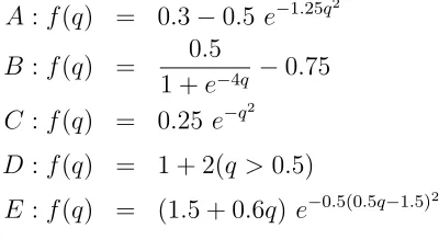
The range of possible functional coefficients we consider for either the intercept or the slope functions is given by

A:f(q) = 0.3₋0.5 e−1.25q2

B :f(q) = 0.5

1 +e−4q −0.75

C :f(q) = 0.25e−q2

D:f(q) = 1 + 2(q >0.5)

E :f(q) = (1.5 + 0.6q) e−0.5(0.5q−1.5)2

(6)

thus covering a very wide range of shapes including for illustration purposes a threshold type function which violates our differentiability assumption. Following standard practice in the functional coefficient literature, the quality of our estimators will be assessed via the computation of the root MSE defined as follows

RM SEi =

v u u t1

k

k

X

r=1

( ˆfi(qr)−fi(qr))2 i= 0,1 (7)

for some qr falling within each bin, say the midpoint (note that since we operate under

piece-wise linearity the location at which we evaluate the function within the bin does not affect its value). All our experiments use N ID(0,1) variables for the random disturbances zt while

setting _{ρu, ρv, ρq}={0.25,0.25,0.25} thus allowing both serial correlation and endogeneity.

Before proceeding with our simulations we give a snapshot of the performance of our es-timators by displaying plots of single realisation based ˆfi(q)′s for i = 0,1 together with their

true counterparts. Figure 1 below presents the plots of the functions corresponding to our for-mulations in A-E across samples of size T=500 and T=2000. The corresponding choice for the number of bins was k=50 and k=100.

The above plots suggest that ˆf1(q) displays a good ability to trace its true counterpart f1(q)

along the chosen domain. Interestingly, our estimator also appears to match its true counter-part closely under scenario D when the chosen functional form has a kink. At this stage it is worth recalling that these figures have been obtained allowing for both serial correlation and endogeneity in the underlying dynamics.

Unlike ˆf1(q) however, the estimator of f0(q) appears to perform poorly overall especially

when the sample size is small. This is not unexpected and stems from the slow convergence of the estimator relative to that of ˆf1(q) as well as its large variance. Regardless of the sample size

the plots make clear the fact that the variance of ˆf0(q) is substantially larger than that of ˆf1(q).

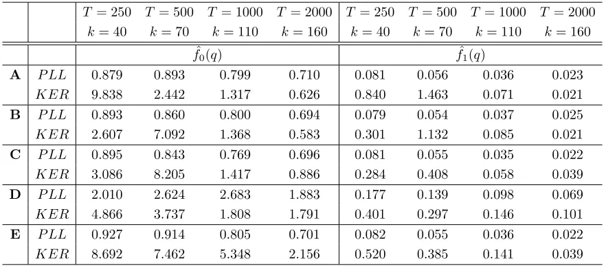
We next aim to highlight more formally the consistency properties of our estimators by documenting the progression of the corresponding RMSEs as the sample size and associated bin number is allowed to increase. Results across a selective set of scenarios are summarised in Table 1 below which displays simulated averages of (7) across N=2000 Monte-Carlo replications. The rows labelledPLLcorrespond to our piecewise local linear estimator while the rows labelled

KER are based on a Kernel estimation as described in Xiao (2009) and using a Gaussian Kernel with h= 1/k (the number of bins associated with each sample size is denoted k).

Table 1. RMSE of Estimators under Serial Correlation and Endogeneity

T = 250 T = 500 T = 1000 T = 2000 T = 250 T = 500 T = 1000 T = 2000

k= 40 k= 70 k= 110 k= 160 k= 40 k= 70 k= 110 k= 160 ˆ

f0(q) fˆ1(q)

A _{P LL 0.879 0.893 0.799 0.710 0.081 0.056 0.036 0.023}

KER 9.838 2.442 1.317 0.626 0.840 1.463 0.071 0.021

B _{P LL 0.893 0.860 0.800 0.694 0.079 0.054 0.037 0.025}

KER 2.607 7.092 1.368 0.583 0.301 1.132 0.085 0.021

C _{P LL 0.895 0.843 0.769 0.696 0.081 0.055 0.035 0.022}

KER 3.086 8.205 1.417 0.886 0.284 0.408 0.058 0.039

D _{P LL 2.010 2.624 2.683 1.883 0.177 0.139 0.098 0.069}

KER 4.866 3.737 1.808 1.791 0.401 0.297 0.146 0.101

E _{P LL 0.927 0.914 0.805 0.701 0.082 0.055 0.036 0.022}

KER 8.692 7.462 5.348 2.156 0.520 0.385 0.141 0.039

Across all functional forms we note a clear decline in the PLL based RMSEs corresponding to ˆ

f1(q) asT andkare allowed to increase. Interestingly and with the exception of scenario D which

is ruled out by our assumptions the average RMSE figures are also very similar acrossT andk. A suitable choice for h or k is an important topic in its own right and merits further research. For our purpose our choice was guided by the requirement thatT h3/2 _{→0 which gave us a rough}

see their RMSEs decline substantially faster than their intercept counterparts. Looking at the RMSE figures corresponing to ˆf0(q) we note their tendency to decline very slowly.

Our comparisons with an alternative Kernel based estimator also suggest that our method works well. Naturally, since alternative Kernels or functional forms may produce different finite sample outcomes it would be misleading to argue that our PLL approach dominates alterna-tive approaches. Indeed our key goal here was to introduce a simple approach to estimating functional coefficients that displays good finite sample properties rather than proposing an al-ternative methodology that aims to dominate existing approaches.

5

Conclusions

APPENDIX

LEMMA 1: As h_→0 (i) E[Irt−1]/h→gq(q), (ii) E[Irt−1(qt−1−q)m] =o(hm+1).

PROOF: We focus on (ii) and evaluate the expression at some q=qr. We have

|E[(qt−1−qr)mIrt−1]| =

Z Hr

(q₋qr)mgq(q)dq

≤ Z Hr

|q₋qr|mgq(q)dq

≤ hm

Z

Hr

gq(q)dq=const∗ hm+1 (8)

and the result follows.

PROOF OF PROPOSITION 1: Given xt, yt, qt and the known bin cutoff locations the least

squares estimators of the interceptβ0r and slope parameterβ1r of the regression line within each

bin can be formulated as

ˆ

β0r = yr−βˆ1rxr

ˆ

β1r =

P

(xt−xr)Irt−1yt

P

(xt−xr)2Irt−1

(9)

with xr = PxtIrt−1/PIrt−1 and yr =

P

ytIrt−1/PIrt−1. Next, using yt = f0(qt−1) +

f1(qt−1)xt+ut, taking a first order Taylor expansion of the unknown coefficients around some

q_∈Hr

fi(qt−1)≈fi(q) +fi′(q)(qt−1−q) +o(h2)

for i= 0,1 and ignoring terms that are o(h2_{) we can rewrite ˆβ} 1r as

ˆ

β1r−f1(q) =

P

(xt−xr)Irt−1[f0(qt−1) +f1(qt−1)xt]

P

(xt−xr)2Irt−1

+

P

(xt−xr)Irt−1ut

P

(xt−xr)2Irt−1

= f′

0(q)

P

(xt−xr)(qt−1−q)Irt−1

P

(xt−xr)2Irt−1

+f′

1(q)

P

xt(xt−xr)(qt−1−q)Irt−1

P

(xt−xr)2Irt−1

+

P

(xt−xr)Irt−1ut

P

(xt−xr)2Irt−1

. (10)

It is now also convenient to reformulate the above as

T√h( ˆβ1r−f1(q)) = f0′(q)

P

(xt−xr)(qt−1−q)Irt−1/T2h

P

(xt−xr)2Irt−1/T2h

T√h+

f′

1(q)

P

xt(xt−xr)(qt−1−q)Irt−1/T2h

P

(xt−xr)2Irt−1/T2h

T√h+

P

(xt−xr)Irt−1ut/T h

P

(xt−xr)2Irt−1/T2h ≡ T√hf′

0(q)Ar+T √

h f′

and the result follows by showing thatT√h Ar and T √

h Br are asymptotically negligible when

T h3/2 _{→ 0 while C}

r is Op(1). Note that the denominators of the above are always bounded in

distribution as T h_{→ ∞}, since

X

xt2Irt−1/T2h−gq(q)

Z B2

v(s)

≤ X

xt2Irt−1/T2h−

X

B_v2(t/T)Irt−1/T h

+ X

B_v2(t/T)Irt−1/T h−gq(q)

Z B_v2(s)

≤ sup t |

Irt−1/h|

X x2t/T

2

−XBv2(t/T)/T

+ sup

s∈[0,1]

Bv(s) + 1

!2

X

Irt−1/T h−gq(q)

. (12)

Using Markov inequality Pr (sup_t|Irt−1/h|> M) ≤ suptE(Irt−1)/M h ≤ supgq(q)/M → 0 as

M _{→ ∞}thereforeIrt−1/his uniformly bounded. Our assumptions also ensure thatPxt2/T2 ⇒

R1

0 B 2

v (see Phillips (1987)) and finally the asymptotic negligibility of the last term in (12) as

T h_{→ ∞} follows from a suitable law of large numbers for strong mixing processes (e.g Hansen (1991, Corollary 4). See also Hansen (2008, Theorem 1)). Similarly for xr.

We have for q_∈Hr,|qt−1−q|< h and f1′(q) bounded,

T√h_|B_{r| ≤} T√h

P

|xt(xt−xr)(qt−1−q)|Irt−1

P

(xt−xr)2Irt−1 ≤ T h3/2

P

|xt(xt−xr)|Irt−1

P

(xt−xr)2Irt−1 →

0 (13)

since T h3/2 _{→0. The asymptotic negligibility of T}√_{h A}

r follows along identical lines using the

fact that

T√h

X

(xt−xr)(qt−1−q)Irt−1/T2h

≤

√

T h3/2max

t≤T

xt √ T X

Irt−1/T h

≤ √T h3/2 sup

s∈[0,1]

Bv(s) + 1

! X

Irt−1/T h (14)

since as before sup_s∈[0,1]Bv(s) + 1 PIrt−1/T his bounded T √

h Ar →0.

Finally, for Cr, usingxt =xt−1+vt we write

P

(xt−xr)Irt−1ut

T√h =

P

xt−1Irt−1ut

T√h +

P

utvtIrt−1

T√h −xr

P

utIrt−1 √

T h . (15)

Notice that Pr

P

utvtIrt−1/T √

h > ε

≤ T h1 E[u2tvt2Irt−1] → 0. Same goes for the term

P

utIrt−1/ √

T h and xr is bounded by sups∈[0,1]Bv(s) + 1

hence the third term is Op(1).

So we can concentrate on P

xt−1utIrt−1/T √

h. We write as before

1

T√h

X

xt−1utIrt−1

≤

sup

s∈[0,1]

Bv(s) + 1

!

1

√

T h

X

and hence leading to the required result.

Proceeding along the same lines for ˆβ0r and using ˆβ1r =f1(q) +Op(1/T √

h) we write

ˆ

β0r−f0(q) = f0′(q)

P

(qt−1 −q)Irt−1

P

Irt−1

+f′

1(q)

P

(qt−1−q)xtIrt−1

P

Irt−1

+

P

utIrt−1

P

Irt−1 −

xrOp(

1

T√h). (17)

Applying suitable normalisations we reformulate (17) as

√

T h( ˆβ0r−f0(q)) = f0′(q)

P

(qt−1−q)Irt−1

P

Irt−1

√

T h+

f′

1(q)

P

(qt−1−q)xtIrt−1

P

Irt−1

√

T h+

P

utIrt−1/ √

T h

P

Irt−1/T h

+Op(1). (18)

Proceeding as above it is again straightforward to observe that under√T h3/2 _{→0 the first two}

terms in the right hand side of (18) are asymptotically negligible while the third term is Op(1)

by our Assumptions A.

REFERENCES

Banerjee, A. N., 1994. A method of estimating the average derivative. CORE Discussion Paper: 9403, Universit´e Catholique de Louvain.

Banerjee, A. N., 2007. A method of estimating the average derivative. Journal of Econo-metrics, 136, 65-88.

Berenguer-Rico, V., 2010. Summability of Stochastic Processes: A Generalization of Inte-gration and Co-inteInte-gration valid for Non-linear Processes, Universidad Carlos III de Madrid Working Paper.

Berenguer-Rico, V. and Gonzalo, J., 2011. Co-Summability: From Linear to Non-Linear Co-Integration, Universidad Carlos III de Madrid Working Paper.

Breitung, J., 2001. Rank tests for nonlinear cointegration, Journal of Business and Economic Statistics, 19, 331-340.

Cai, Z., Li, Q. and Park, J. Y., 2009. Functional Coefficient Models for Nonstationary Time Series Data, Journal of Econometrics, 148, 101-113.

Chen, R. and Tsay, R.S., 1993. Functional Coefficient Autoregressive Models, Journal of the American Statistical Association, 88, 298-308.

Fan, J. and Zhang, W., 1999. Statistical Estimation in Varying Coefficient Models, The Annals of Statistics, 27, 1491-1518.

Fan, J. and Yao, Q., 2003. Nonlinear Time Series. Springer-Verlag, New-York.

Gonzalo, J. and Pitarakis, J., 2006. Threshold Effects in Cointegrating Relationships, Oxford Bulletin of Economics and Statistics, 68, 813-833.

Granger, C.W.J. and Hallman, J., 1991. Nonlinear Transformations of Integrated Time Series, Journal of Time Series Analysis, 12, 207-234.

Hansen, B., 1991. Strong Laws for Dependent Heterogeneous Processes, Econometric The-ory, 7, 213-221.

Hansen, B., 2008. Uniform Convergence Rates for Kernel Estimation with Dependent Data, Econometric Theory, 24, 726-748.

Hastie, T. J. and Tibshirani, R. J., 1993. Varying Coefficient Models, Journal of the Royal Statistical Society, Series B, 55, 757-796.

Juhl, T., 2005. Functional-Coefficient Models under Unit Root Behaviour, Econometrics Journal, 8, 197-213.

Karlsen, H. A., Myklebust, T. and Tjostheim, D., 2007. Nonparametric estimation in a nonlinear cointegration type model, Annals of Statistics, 35, 252-299.

Kasparis, I. and Phillips, P. C. B., 2009. Dynamic Misspecification in Nonparametric Coin-tegrating Regression. Yale University Working Paper

Phillips, P.C.B., 1987. Time series regression with unit roots, Econometrica, 55, 277-302.

Saikkonen, P. and Choi, I., 2004. Testing linearity in cointegrating smooth transition regres-sions, Econometrics Journal, 7, 341-365.

Senturk, D. and Mueller, H. G., 2005. Covariate-adjusted regression. Biometrika, 92, 75-89.

Senturk, D. and Mueller, H. G., 2006. Inference for covariate adjusted regression via varying coefficient models. Annals of Statistics, 34, 654-679.

Wang, Q. and Phillips, P.C.B., 2009. Structural Nonparametric Cointegrating Regression, Econometrica, 77, 1901-1948.