Changes in energy efficiency in Australia: A decomposition of aggregate energy intensity using Logarithmic Mean Divisia approach

Munich Personal RePEc Archive

Changes in energy efficiency in Australia:

A decomposition of aggregate energy

intensity using Logarithmic Mean Divisia

approach

Shahiduzzaman, Md and Alam, Khorshed

School of Accounting, Economics Finance, Australian Centre for

Sustainable Business Development, University of Southern

Queensland

January 2012

Online at

https://mpra.ub.uni-muenchen.de/36250/

1

Changes in energy efficiency in Australia: A decomposition of aggregate

energy intensity using Logarithmic Mean Divisia approach

Md Shahiduzzaman*

School of Accounting, Economics & Finance and Australian Centre for Sustainable Business & Development

University of Southern Queensland, Australia

Khorshed Alam

School of Accounting, Economics & Finance and Australian Centre for Sustainable Business & Development

University of Southern Queensland, Australia

Abstract

This paper provides an empirical estimation of energy efficiency and other proximate factors that explain energy intensity in Australia for the period 1978-2009. The analysis is performed by decomposing the changes in energy intensity by means of energy efficiency, fuel mix and structural changes both at sectoral and sub-sectoral levels of the economy. Results show that the driving forces behind the decrease in energy intensity in Australia are efficiency effect and sectoral composition effect, where the former is found to be more prominent than the latter. Moreover, the favourable impact of the composition effect has been consistently slowed down in the recent past. A perfect positive association characterizes the relationship between energy intensity and carbon intensity in Australia. Given the trends in decomposition factors, it is necessary to boost energy efficiency further to reduce Australia’s overall contribution to energy intensity and carbon emissions in the future.

Key words: Energy intensity; Energy efficiency; Index decomposition analysis

*

Corresponding author. Tel.: 61 0458823191; fax: 61 7 46315597

Email addresses: [email protected] (M. Shahiduzzaman),

2

Changes in energy efficiency in Australia: A decomposition of aggregate

energy intensity using Logarithmic Mean Divisia approach

1. Introduction

As energy accounts for the largest share of greenhouse gases (GHG) emissions1, contemporary energy and environmental policies consider energy efficiency to be at the forefront of policy objectives (Ang 2006; IEA 2008; Kanako 2008; Wilson et al. 1993). In retrospect, the recent policy document on climate change in Australia affirmed the need of improving energy efficiency as one of the key elements to reduce the country’s carbon emissions (Commonwealth of Australia 2011). In the European Union (EU) countries, while carbon pricing and specific renewable energy targets are in place, a separate target has also been set to reduce energy consumption by 20% in 2020 through the improvement of energy efficiency (EU 2008). In several summits (2005 in Gleneagles, 2006 in St Petersburg, and 2007 in Heiligendamm), the leaders of group of eight (G8) avowed the role of energy efficiency in both advanced and emerging economies to combat climate change, which has further been reinforced in the 2009 G8 Summit in L'Aquila. A separate policy to improve energy efficiency is required in order to correct for the associated market failure related to energy efficiency and to encourage cost-effective energy efficiency actions (Ryan et al. 2011).

In the context of designing appropriate policies, a clear exposition of the present state of energy efficiency and its historical trend would be of foremost importance. Energy efficiency trends need to be monitored at both aggregate economy and end-use levels, while the achievement of policies may be evaluated in terms of national aggregates. This requires the use of a single framework that can adequately capture the perspectives on energy

1

3

efficiency changes from end-use to aggregate level. Nonetheless, the measurement of energy efficiency is not that straight forward at the aggregate level as it is at the lower level of aggregation. As for example, at the most refined level of disaggregation, energy efficiency can simply be defined as an inverse of changes in energy intensity (energy per unit of monetary or physical activity2).However, this simple measurement of energy efficiency may not be applicable at the aggregate level as there are some other factors than efficiency, such as structural changes, which could contribute to the observed changes in energy intensity. For example, if the composition of the economy changes over time from energy intensive industrial sector to the less energy intensive service sectors, energy intensity can decline notably without any change in energy efficiency. Similarly, at an early stage of economic development, shifts from low energy intensive sector, such as agriculture to high energy intensive industrial sector can lead the energy intensity to increase. Similarly, energy intensity could be affected by the changes in fuel mix due to the differences in economic productivity among different energy types (Ma & Stern 2008). It is, therefore, necessary to find an appropriate method that can separate out the energy efficiency trends from other proximate determinants of the aggregate energy intensity. Decomposition method can be used as a suitable tool in this case as it accurately separates energy efficiency from the factors unrelated to the efficiency at a given level of disaggregation, for example, at the sub-sectoral/end-use levels (Ang & Zhang 2000). The economy-wide energy efficiency trend is thus derived using a bottom-up framework, providing a meaningful interpretation (Ang 2006).

This paper provides an empirical estimation of energy efficiency trends and other proximate factors that explain energy intensity in Australia for the period 1978-2009 by applying the Index Decomposition Approach (IDA), more specifically, the Log Mean Divisia

2

4

Index (LMDI) technique. Another branch of IDA is the Arithmetic Mean Divisia Index (AMDI) method, which has been dominantly used in the earlier studies in Australia (Cox et al. 1997; Harris & Thorpe 2000; Tedesco & Thorpe 2003; Wilson et al. 1993). In recent years, there are some studies at Australian Bureau of Agricultural and Resource Economics – Bureau of Rural Science (ABARE-BRS) those have used the LMDI approach (Petchey 2010; Sandu & Petchey 2009; Sandu & Syed 2008). Sandu and Syed (2008) and earlier studies made use data for relatively aggregate level, while most recent studies (Petchey 2010; Sandu & Petchey 2009) have employed data at more disaggregate levels. Theoretically, the more disaggregated the series is, the more accurate the energy efficiency measure is due to less mix-up of heterogeneous nature of the output at the lower level (Ang 2006; Petchey 2010). This study complements the recent trend is literature in four mains aspects. Firstly, the time series used in this study is considerably longer: 1989-90 to 2006-07 used by Sandu and Petchey (2009) and 1989-90 to 2007-08 by Petchey (2010) as compared to 1977-78 to 2008-09 utilized in this study. The use of longer time series enabled us to monitor the trend of energy intensity, energy efficiency and structural factors aftermath the oil crisis in 1970s along with the changes in recent years, therefore providing rich set of perspectives. Secondly, this study included the fuel mix effect in the decomposition, which has not been covered in the recent decomposition studies. Thirdly, added focus has been given to the electricity generation sub-sector, which is at the core of CO2 emissions problem in Australia. Finally, a

succinct review of the decomposition literature in Australia in the area of energy and environmental has been provided.

5

methodology and data, Section 5 presents and discusses the decomposition results, and finally, Section 6 presents conclusions.

2. Overview of Australia’s energy intensity

2.1 Historical trend

While Australia experienced an overall decline in annual average growth of total energy consumption over the last four decades, average growth in energy consumption remained relatively unchanged in the 1980s and 1990s (Table 1). Nonetheless Gross Domestic Product (GDP) grew, on average, at a faster rate and remained above the growth rate of energy consumption since 1980s (Table 1). During 2001-2009, GDP growth rate in Australia was about 1.46 percentage point higher than the growth of total energy consumption. The pattern reflects a decreasing energy intensity trend in the Australian economy in the last three decades, with a substantial improvement in the most recent periods.

6

Table 1: Annual growth of energy consumption in Australia

1974-1980

1981- 1990

1991- 2000

2001- 2009

1974- 2009

% % % % %

Agriculture 3.34 1.76 2.65 3.45 2.80

Mining 5.32 7.47 5.53 5.48 5.95

Manufacturing 0.84 1.1 1.13 0.63 0.93 Electricity generation 6.54 3.73 2.99 2.28 3.89 Construction 7.08 0.93 -3.51 -1.12 0.85 Transport 3.15 2.09 2.28 1.41 2.23 Services a 3.59 3.78 3.78 2.66 _3.45 Residential 2.15 2.12 1.98 1.15 1.85

Other b 0.96 0.57 1.19 0.01 _0.68

All sectors 3.06 2.37 2.34 1.68 2.36 GDP growth rate c 2.78 3.01 3.45 3.14 _3.10 Population growth rate 1.2 1.5 1.2 1.5 1.4

Notes: a

Includes ANZSIC Divisions F, G, H, J, K, L, M, N, O, P, Q and the water, sewerage and drainage industries. b

Includes consumption of lubricants and greases, bitumen and solvents, as well as energy consumption in the

gas production and distribution industries. c

Growth of Industry Gross Value Added, Chain Volume measures, reference year 2008-09.

Sources: ABARE (2009); Cat no 5206.0 Australian National Accounts: National Income, Expenditure and

Product, Table 33. Industry Gross Value Added, Chain volume measures, Annual, Australian Bureau of

Statistics. Cat no 3105: Australian Historical Population and Cat no 3101.0: Australian Demographic Statistics,

Australian Bureau of Statistics.

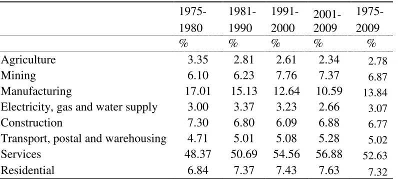
Table 2: Sectoral share to GDP a

1975- 1981- 1991- 2001-

2009

1975- 1980 1990 2000 2009

% % % % %

Agriculture 3.35 2.81 2.61 2.34 2.78

Mining 6.10 6.23 7.76 7.37 6.87

Manufacturing 17.01 15.13 12.64 10.59 13.84

Electricity, gas and water supply 3.00 3.37 3.23 2.66 3.07

Construction 7.30 6.80 6.09 6.88 6.77

Transport, postal and warehousing 4.71 5.01 5.08 5.28 5.02

Services 48.37 50.69 54.56 56.88 52.63

Residential 6.84 7.37 7.43 7.63 _7.32

a

7

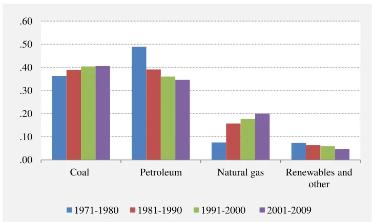
“Electricity generation”, “Transport” and “Manufacturing” are the three dominant sectors of Australia’s total energy consumption, together representing about 78 percent of total energy consumption during 2001-2009 (Table 3). While growth of energy use declined steadily for the “Electricity generation” sector over the last three decades (Table 1), its share to total energy consumption increased substantially from 21 percent during 1974-1980 to about 30 percent during 2001-2009 to support the growing demand for electricity in the economy (Table 3). The increasing share of the “Electricity generation” sector to total energy consumption resulted in an increasing use of coal in the primary energy mix over the last four decades (Figure 1). On the other hand, both energy growth (Table 1) and share to total energy consumption (Table 3) declined gradually for the “Manufacturing” and “Transport” sectors over the same period of time. In the “Manufacturing” sector, annual growth of energy consumption increased in the 1980s and 1990s (Table 1), despite its declining output share to GDP (Table 2). In the “Services” sector, average growth of energy consumption remained unchanged in the 1980s and 1990s, while the output contribution of the sector increased steadily over the period of time (Table 2). The contribution of “Services” sector stood about 57 percent of GDP but only about 5 percent of total energy consumption during 2001-2009. “Manufacturing”, however, constituted, about 23 percent of total energy consumption for all sectors of the economy as compared to about 11 percent share to GDP during 2001-2009 (Table 3). The declining share (output) of “Manufacturing” and increasing share of “Services” over the period postulate the sectoral shift of the Australian economy.

8

Table 3: Sectoral composition of total energy consumption

1974-

1980

1981- 1990

1991- 2000

2001- 2009

1974-2009

% % % % %

Agriculture 1.46 1.58 1.43 1.7 1.54

Mining 2.46 2.88 4.97 6.28 4.15

Manufacturing 33.18 27.83 25.51 23.09 27.40 Electricity generation 21.12 26.44 27.42 30.11 26.27 Construction 1.13 1.07 0.74 0.5 0.86 Transport 26.33 26.41 25.7 24.72 25.79 Services a 3.26 3.56 4.16 4.6 _3.90 Residential 8.85 8.36 8.18 7.53 8.23

Other b 2.16 1.86 1.58 1.46 _1.77

Total 100 100 100 100 100

a _{Includes ANZSIC Divisions F, G, H, J, K, L, M, N, O, P, Q and the water, sewerage and}

drainage industries.

b

Includes consumption of lubricants and greases, bitumen and solvents, as well as energy consumption in the gas production and distribution industries.

Source: ABARE (2009)

Figure 1: Changes in fuel mix in total energy consumption

Notes: “Renewables and other” includes hydro electricity, wind, solar, Bio-fuel, wood & wood-waste and Bassage.

Source: Author’s compilation using data from Australian energy consumption by fuel, Table C, ABARE (2009).

.00 .10 .20 .30 .40 .50 .60

Coal Petroleum Natural gas Renewables and other

9

2.2 Australian’s energy intensity as compared to the international standard

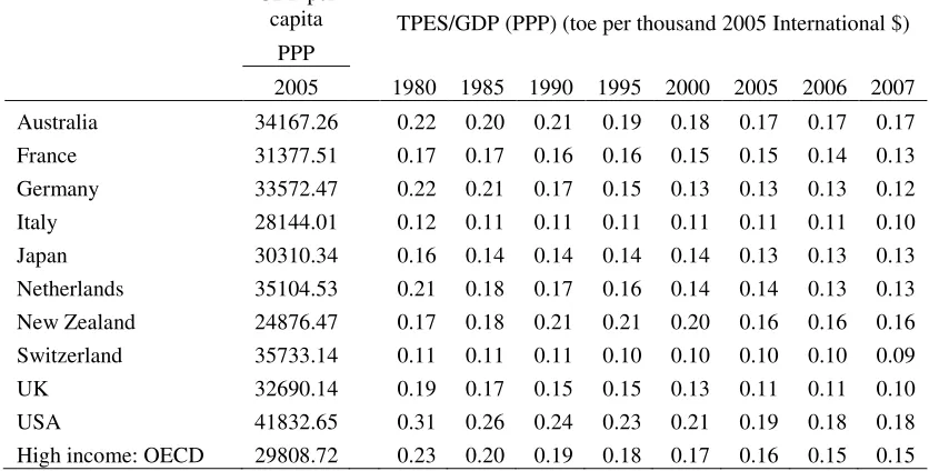
While Australia achieved a decline in aggregate energy intensity over the last few decades, its achievement is relatively weaker as compared to the competing advanced countries. As shown in Table 4, aggregate energy intensity in Australia remained well above the one in OECD countries since 1990s. Indeed, most OECD countries experienced a steady decline in energy intensity following the oil prices shock in mid-1970s, which continued in the subsequent decades. Australia, on the other hand, experienced an increase in energy intensity during the period of 1970-1977 before experiencing a fairly strong decline until the mid-1980s. The declining trend of energy intensity in Australia then discontinued until the early 1990s but again experienced a gradual decline through the 1990s to recent times.

Table 4: Ratio of total primary energy supply (TPES) to GDP in Australia as compared to selected advanced countries

GDP per

capita _{TPES/GDP (PPP) (toe per thousand 2005 International $)} PPP

2005 1980 1985 1990 1995 2000 2005 2006 2007

Australia 34167.26 0.22 0.20 0.21 0.19 0.18 0.17 0.17 0.17 France 31377.51 0.17 0.17 0.16 0.16 0.15 0.15 0.14 0.13 Germany 33572.47 0.22 0.21 0.17 0.15 0.13 0.13 0.13 0.12 Italy 28144.01 0.12 0.11 0.11 0.11 0.11 0.11 0.11 0.10 Japan 30310.34 0.16 0.14 0.14 0.14 0.14 0.13 0.13 0.13 Netherlands 35104.53 0.21 0.18 0.17 0.16 0.14 0.14 0.13 0.13 New Zealand 24876.47 0.17 0.18 0.21 0.21 0.20 0.16 0.16 0.16 Switzerland 35733.14 0.11 0.11 0.11 0.10 0.10 0.10 0.10 0.09 UK 32690.14 0.19 0.17 0.15 0.15 0.13 0.11 0.11 0.10 USA 41832.65 0.31 0.26 0.24 0.23 0.21 0.19 0.18 0.18 High income: OECD 29808.72 0.23 0.20 0.19 0.18 0.17 0.16 0.15 0.15

a

Constant 2005 international $.

Source: Authors’ elaboration of data from the World Bank (2010).

10

sharply than that in Australia. A similar trend is also witnessed in the case of Germany, which experienced a very similar level of energy intensity to Australia in the early 1970s, which, however, was followed by a considerably steeper decline in the last four decades (Table 1). Given the trends, Australia’s energy intensity remained well above the most advanced countries’ in the last three decades. Australia, therefore, needs to have a substantial improvement of energy efficiency to keep pace with the advanced countries.

Figure 2: Trends of aggregate energy intensity: Australia vs. USA

Notes: Energy intensity calculated as the ratio of total primary energy consumption (toe per thousand 2005 International $) against GDP (PPP constant 2005 international $).

Source: Authors’ elaboration of data from the World Bank (2010).

Focacci (2003) found that falling energy intensity has historically been accompanied by reducing CO2 intensity in Italy, Japan, UK and USA. In case of Australia, the country does

not seem to have experienced any significant reduction in either energy intensity or CO2

emissions intensity in the 1980s and 1990s (Focacci 2003). Geller et al. (2006) reported that the Australia’s reduction in energy use per unit of GDP and improvement of energy efficiency (i.e., energy intensity effect as seen in Fig 2) is relatively lower than the major OECD countries.

.10 .15 .20 .25 .30 .35

11

3. Review of literature

A rich body of literature has emerged employing decomposition method in energy and environmental analysis since 1980s (see, Ang & Zhang 2000, for a survey ). Early studies mostly focused on the industrial energy consumption (Park et al. 1993), while the recent trend has been to extend the analysis to an economy-wide level by appropriately combining sectoral and sub-sectoral data (Greening et al. 1997; Ma & Stern 2008; Petchey 2010; Sandu & Petchey 2009). While the relative roles of the efficiency effect and structural effect are country specific (Greening et al. 1997), the literature places emphasis on the efficiency effects in reducing energy intensity, especially in the advanced countries’ cases (IEA 2004). In case of Australia, Wilson et al. (1993) utilized the AMDI method, which has been later replicated in other studies in subsequent years to examine energy intensity or efficiency trends in Australia (Cox et al. 1997; Harris & Thorpe 2000; Tedesco & Thorpe 2003). More recently, Sandu and Syed (2008), Sandu and Petchey (2009) and Petchey (2010) have applied the LMDI approach to decompose end use energy intensity in the Australian economy. On the other hand, Wood (2009) adopted the structural decomposition analysis (SDA) to examine the impacts of industrial efficiency and other proximate factors on changes in greenhouse gas emissions in Australia.3

The results from the previous studies are mixed with respect to the relative importance of the real intensity effects and composition effects on changing energy intensity. Wilson et al. (1993) and Cox et al. (1997) found the role of real intensity to be dominant in changing aggregate energy intensity in Australia. On the other hand, in a relatively recent study, Tedesco and Thorpe (2003) found that structural factors (e.g., reduction of energy intensive

3

The difference between IDA and SDA is that the latter uses an input-output model, which can be applied to a given set of energy and production data at any level of aggregation. These two methods have been developed independently in the literature and pose distinct advantages and focus. Interested readers can consult Hoekstra and van den Bergh (2003) for a comparison between them.

12

13

large positive fuel share effect using the AMDI approach. On the other hand, in the case of perfect decomposition by a LMDI approach, the fuel share effect was found to be small and negative (Hatzigeorgiou et al. 2008). Therefore, the measurement of fuel mix effect in the previous studies in Australia could be distorted due to the use of an AMDI approach as it provides imperfect decomposition. In recent studies in Australia, i.e., Sandu and Syed (2008), Sandu and Petchey (2009) and Petchey (2010) did not include the role of fuel mix effects in the decomposition analysis.

4. Methodology and data

14

Divisia, such as AMDI and LMDI. As discussed by Ang (2004), while both AMDI and LMDI approaches satisfy the time reversal test, LMDI is the only approach out of the two that satisfies the Fisher’s (1922) factor reversal test (Ang & Zhang 2000; Sato 1976). From an application point of view, both AMDI and LMDI approaches pose computational problems with zero values as they are based on log changes. This is particularly true when different fuel vectors are included in the analysis to examine the fuel mix effects. This is quite common that the consumption of a particular fuel type is not observed for one or more periods in an economic sub-sector. This problem can be handled by substituting the zero values with a small positive number, for example, something between 10ିଵ଴ _and 10ିଶ଴_,

therefore finding converging results as the small number approaches zero (Ang & Choi 1997; Choi & Ang 2001, 2002). In case of some previous studies in Australia as cited above, the zero values were replaced by 10ି଺_{(Harris & Thorpe 2000; Tedesco & Thorpe 2003).}

However, as shown in Ang and Choi (1997), the AMDI method may not lead to a converging result. In contrast, the converging results are guaranteed in case of a LMDI approach (Ang & Choi 1997; Ang & Liu 2007). Therefore, LMDI approach is preferred than the other methods of decomposition (Ang 2004). As articulated by Ang (2004), the LMDI is the “best” decomposition method providing complete decomposition results with no residual among various alternatives commonly used in the literature. Therefore, our selection of the LMDI as the decomposition method is not arbitrary, rather based on the virtue of the methodological superiority.

4.1 Model

Suppose, an economy is composed of various sectors and sub-sectors, and energy consumption in subsector k is denoted as Ek. We can therefore write

Q Q Q

Q Q Q E

E j

j k k k

15

Where, Q represents aggregate output. Qk and Qj denote output of subsector k and sector j,

respectively.

Energy consumption at sector j, Ej is the aggregation of the sub-sectoral level of

energy consumption within the sector,

∑

Similarly, energy consumption at the aggregate economy E is the sum of energy consumption by various sectors.

∑

Combining, (1) through (3):

Q Q Q Q Q Q E E j j k j k k

k ⋅ ⋅ ⋅

=

∑∑

Dividing both side of the equation (4) by Q, we can write,

Q Q Q Q Q E Q E j j k j k k

k ⋅ ⋅

=

∑ ∑

Where, Q

E

represents the aggregate energy intensity (I) of the economy.

Incorporating fuel mix effect, equation (5) can be modified as:

Q Q Q Q Q E E E I j j k k k j k m k

km ⋅ ⋅ ⋅

=

∑∑∑

where, m denotes the fuel vectors in total energy consumption of subsector k . Equation (6) can be symbolized as

j k k j k m

m I S S

S

I =

∑ ∑ ∑

Where, Sm is the share of fuel m in total energy consumption of subsector k, Ik represents real

intensity, i.e., energy intensity at the subsector k, Sk is the output share of a subsector k to

16

Differentiating equation (7) with respect to time yields,

j k k j k m

m j

k k j k m

m j

k k j k m

m I S S S I S S S I S S

S

I&=

∑ ∑ ∑

∑ ∑ ∑

∑ ∑ ∑

j k k j k m

m I S S

S ⋅ ⋅ ⋅ &

+

∑ ∑ ∑

Writing equation (8) in terms of growth rates and integrating,

dt g dt g dt g

I t _jkm

j k m Sk jkm

t

j k m Ik t

j k m

jkm

sm⋅ + ⋅ ⋅ + ⋅ ⋅

=

∆

_{∫ ∑∑∑}

_{∫ ∑∑∑}

_{∫ ∑∑∑}

0 0 0 . dt g _jkm t

j k m

Sm⋅ ⋅

∫ ∑∑∑

0 (9)

where,

ω

(1976) weighting scheme, where logarithmic mean is used as a weight function. According

to Sato-Vartia, the weight function f can be specified as4:

) ln /(ln ) ( ) ,

(

ϕ

γ

γ

ϕ

γ

ϕ

∫ , for γ ≠ϕ (10)

Where

ϕ

ω

γ

ω

Using the notations of equation (10), equation (9) becomes,

) ln )(ln , ( ) ln )(ln ,

( ₀ k₀

j k m

kt m

j k m

mt S I I

S

I = − + −

∆

∑∑∑∫

ϕ

γ

∑∑∑∫

ϕ

γ

) ln )(ln

,

( _k0

j k m

kt S

S −

∑∑∑∫

ϕ

γ

j k m

jt S

S −

∑∑∑∫

ϕ

γ

Equation (11) is the additive LMDI specification, which can be denoted as:

strs strss

eff

fm I I I

I

I =∆ +∆ +∆ +∆

∆ (12)

where, ∆ represents the total intensity effect, ∆Ifm is the intensity change due to change in

fuel mix and Istrss, Istrs and ∆Istri represent total intensity change due to structural change at

subsector and sector level, respectively.

4

17

The above model is a complete decomposition model and can be applied when

sub-sectoral data for economic sectors are available.

4.2 Data

Our decomposition is based on two levels of industrial disaggregation comprising 8

sectors and 14 sub-sectors of the Australian economy. The sectors are – “Agriculture, forestry

and fishing (division A)”, “Mining (division B) 5”, Manufacturing (division C)”, “Electricity,

gas and water services (division D)” and “Construction (division E)”, “Commercial and

services (divisions F, G, H, J, K, L, M, N, O, P, Q)”, “Transport, postal and warehousing”

(division I) and “Residential” sectors. We take rent of the residential sectors - gross value

added for “Ownership of dwellings” - as output of the residential sector. The sub-sectoral

disaggregation is made in the case of “Manufacturing”, “Electricity, gas and water services”

and “Transport and storage” sectors. The sub-sectors in the “Manufacturing” sector are

categorized as – “Petroleum, coal, chemical and associated products”, “Food, beverage and

tobacco products”, “Textile, clothing, footwear and leather”, “Wood, paper and printing”,

“Non-metalic mineral products”, “Metal products” and “Machinery and equipment”.

Subsectors in “Electricity, gas and water services” are categorized as – “Electricity

generation and supply”, “Gas Production and distribution” and “Water supply and Waste

services”. Sub-sectoral categories in “Transport, postal and warehousing” are “Road

transport”, “Rail, pipeline and other transport, “Air and space transport” and “Other transport

and storage”. The level of disaggregation and the sample chosen in the study are based on the

best available data and consistent series for fuel vectors and output. The fuel vectors included

in the study are coal, petroleum, natural gas, electricity and others. The sample period for the

study is 1978-2009. Data for energy consumption are collected online from the ABARE

(2009) (Table F, Australian energy consumption, by industry and fuel type) and ABS (Table

5

18

33, Cat no 5206.0, Australian National Accounts: National Income, Expenditure and

Product). Energy consumption data are in Gaga joule and Industry Gross Value Added data

are in million Australian dollars in Chain volume measures (reference year 2007-08).

5. Decomposition results and discussions

5.1 Energy intensity in total energy consumption

The complete decomposition of the changes in aggregate energy intensity change in

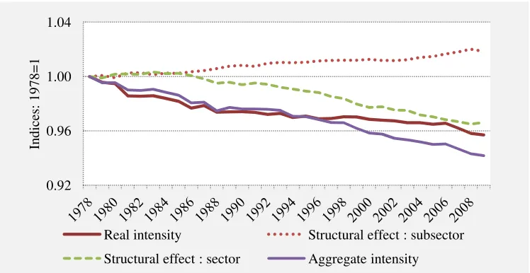
Australia for the sample period is presented in Appendix A. Figure 3 shows the trends of

indices of various underlying factors that govern energy intensity function. As seen in the

figure, real intensity dropped sharply in the 1980s indicating an improvement of energy

efficiency during the period. Real intensity remained below the aggregate energy intensity

trend until mid-1990s. Since then, for most of the 1990s and until recently, energy efficiency

did not experience a notable improvement leaving the real intensity trend well above the

trend of aggregate energy intensity. These results are mostly consistent with earlier studies in

Australia (Cox et al. 1997; Tedesco & Thorpe 2003; Wilson et al. 1994). Wilson et al.(1994)

noted the significant contribution of energy efficiency in decreasing and increasing aggregate

intensity during 1978-1986 and 1986-1991, respectively.

Figure 3: Trends of decomposition factors of changes in total energy intensity

Sources: Authors’ estimation. 0.92

0.96 1.00 1.04

In

d

ic

es

:

1

9

7

8

=

1

Real intensity Structural effect : subsector

19

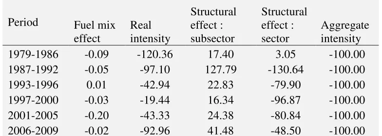
Table 5: Decomposition results for the changes in aggregate energy intensity: aggregated for different periods

Period _{Fuel mix}

effect

Real intensity

Structural effect : subsector

Structural effect : sector

Aggregate intensity

1979-1986 -0.09 -120.36 17.40 3.05 -100.00

1987-1992 -0.05 -97.10 127.79 -130.64 -100.00

1993-1996 0.01 -42.94 22.83 -79.90 -100.00

1997-2000 -0.03 -19.44 16.34 -96.87 -100.00

2001-2005 -0.20 -43.33 24.38 -80.84 -100.00

2006-2009 -0.02 -92.96 41.48 -48.50 -100.00

Notes: Figures exhibit changes in the decomposed factors in terms of changes in aggregate

intensity. Negative numbers represent the positive (favourable) contribution of reducing

aggregate energy intensity. The opposite is true for the positive numbers.

Source: Authors’ estimation.

Our results indicate that the decline in real intensity was about 33% higher than the

decline in aggregate intensity during 1978-1986 (Table 5). During 1978-1986, changes in fuel

mix helped to reduce overall intensity, while structural changes at both sectoral and

sub-sectoral levels posed as barriers to reducing aggregate energy intensity. From 1987 to 1992,

decline in aggregate intensity was attributed to the significant decline of real intensity and

sectoral shift of the economy as the tertiary services sector started to play the dominant role

in industry composition. On the other hand, sub-sectoral composition partly played negative

roles in reducing energy intensity. The result is consistent with Cox et al. (1997). Note that

the sub-sectoral shifts in this analysis only reflect the sub-sectoral shifts of the three most

energy intensive sectors of the economy, i.e., “Manufacturing”, “Transport, postal and

warehousing”, and “Electricity, gas, water and waste services” only. Throughout the sample

period, changes in fuel mix provided some impetus in reducing aggregate intensity but its

overall contribution was very small in most periods except 2000-2005, where large increase

in the petroleum prices led to the reduction of energy consumption in some sub-sectors (e.g.,

20

contribution of fuel mix effects in declining energy intensity since mid-1980s.6 In a recent

study on China applying a LMDI approach, Ma and Stern (2008) also found little

contribution of fuel mix in declining energy intensity over the period 1994-2003.

The bright picture of reducing real energy intensity or improving of energy intensity

during the 1980s has gloomed significantly in most part of the 1990s and up until mid-2000s

in Australia. As pointed out by Tedesco and Thorpe (2003), this dismal picture may

correspond to the era of lower energy prices preceding the oil price shock in the 1970s.

Historically, real prices of coal continued to decline in most part of the 1990s and in the early

2000s. During the period, the dominant contribution of the reduction of aggregate energy

intensity came from the changes in sectoral composition of the economy. The sectoral share

of the Services sector to GDP increased by around 4 percentage points from 1980s to 1990s

(Table 2). During most recent years (2005-2009) energy efficiency improved again to reduce

energy intensity.

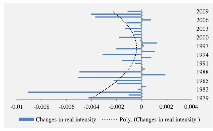
Figure 4: Yearly changes of real intensity: 1978-2009

Note: Negative value indicates decreasing energy intensity

Source: Authors’ estimation.

6

Note that these studies use useful energy measure, which is calculated by multiplying the delivered energy (the energy content) by arbitrarily fixed conversion efficiency for a fuel type. In this study, we also applied the fixed conversion efficiency as used by Wilson et al. (1993) and the subsequent studies in Australia, but found qualitatively similar results.

-0.01 -0.008 -0.006 -0.004 -0.002 0 0.002 0.004 1979 1982 1985 1988 1991 1994 1997 2000 2003 2006 2009

21

Figure 5: Yearly changes in sectoral composition: 1978-2009

Note: Negative value indicates decreasing energy intensity.

Source: Authors’ estimation.

Figure 4 and Figure 5 plot the yearly changes in real intensity and sectoral

composition and their effects on energy intensity. As indicated by the negative values, most

of the changes in real intensity have led to declines in aggregate intensity but the contribution

has reduced significantly in the 1990s. The fitted (polynomial) curve indicates the

improvement of energy efficiency in recent years. This could be associated with the increase

in energy prices in the recent past, growing concerns on environmental issues and incentive

mechanisms of the government. Several potential downside risk factors could be identified.

As seen in Figure 4, energy efficiency deteriorated in 2009 and was even reversed in 2006.

Secondly, the robust contribution of the changes in sectoral composition on the reduction of

energy intensity is most likely to be slowed significantly in the forthcoming years. Thirdly,

fuel mix effects have historically played a smaller role in reducing energy intensity. Given

the trends, it is necessary to improve energy efficiency further to reduce Australia’s overall

contribution to energy intensity in the future.

-0.005 -0.004 -0.003 -0.002 -0.001 0 0.001 0.002 0.003 0.004 1979 1982 1985 1988 1991 1994 1997 2000 2003 2006 2009

22

In terms of net changes, real intensity attributed to 73 percent and sectoral share

attributed to 57 percent of the total changes in aggregate energy intensity during 1978 to

2009. This suggests that energy efficiency has been the dominant factor in reducing energy

intensity in Australia during the sample period in the study.

5.2 Energy intensity in the final energy use

As total energy consumption entails energy consumption in the conversion sectors as well

as energy consumption in the end-use sectors of the economy, it would be worthwhile to

distinguish the trend of end-use energy intensity from that of total energy intensity to gauge

the energy efficiency trends in final energy use. In order to do this, we excluded coal products

from the “Electricity generation subsector”, petroleum from “Petroleum, coal, chemical and

associated products” sub-sector and gas products from “Gas production subsector”. The trend

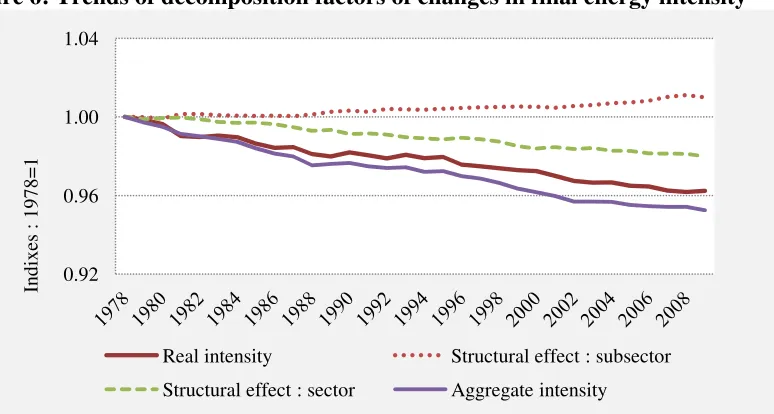
of indices of the decomposition factors are displayed in Figure 6. Some interesting findings

are emerged from the trends of decomposed factors in final energy use. First, unlike Figure 3,

no sharp decline of real intensity was observed during 1980s. The change in real intensity is

seen as less profound than the change in aggregate intensity during the sample period.

Second, with some usual fluctuations, real intensity in final energy use remained relatively

unchanged during 1989-1995. Third, real intensity in final energy use declined steadily since

1995 but at a lower rate than aggregate intensity. Fourth, sectoral shift continued to produce

favourable effects in reducing aggregate intensity since 1978. Finally, similar to total energy,

fuel mix provided the smallest effect on the changes in final energy intensity (Appendix B).

The decomposition results for final energy consumption by aggregating for different periods

23

Figure 6: Trends of decomposition factors of changes in final energy intensity

Source: Authors’ estimation.

5.3 Energy efficiency to limit carbon pollution

A fundamental fact about Australia’s energy consumption is the dominance of carbon

intensive coal and oil products over gas and renewable (Figure 1). Coal and oil together

constitutes about three fourth of total energy consumption in Australia. Therefore, the story

of Australia’s energy consumption is basically a story of carbon intensive fossil fuels

consumption, where coal has remained as a key source of total energy supply, representing an

average of 41 percent share in total energy consumption during 2001-09. Energy related

emissions attributed to about 91 percent of national CO2 emissions and 74 percent of

national GHG emissions in Australia in 2009 (DCCEE 2011). Given the high energy intensity

and carbon intensity of the energy use, Australia ranks among the top twenty polluting

countries of the world with its per capita carbon pollution remaining above the level of any

other developed countries. Despite the close association between energy consumption and

carbon pollution, energy policy and climate change policy in Australia have historically been

characterized by conflicting objectives and separate paths (Riedy 2005). Energy policy has

traditionally been developed to maximise economic return by ensuring abundant supply and 0.92

0.96 1.00 1.04

In

d

ix

es

:

1

9

7

8

=

1

Real intensity Structural effect : subsector

24

lowering energy prices (DPMC 2004).7 Yet, abundant and low-cost energy has lifted carbon

pollution level of the country as compared to the global standard. Only in recent years, a

significant progress has been achieved to unify the two policies to achieve clean energy

future of the country. The Department of Climate Change, established on 3 December 2007,

has been reorganized as the Department of Climate Change and Energy Efficiency in April

2011. Improvement of energy efficiency has now become an important element of reducing

carbon pollution in Australia (Commonwealth of Australia 2011).

Figure 7: Trend of energy intensity and CO2 intensity in Australia

Notes: Energy (kilo tonne of oil equivalent) intensity and CO2 (Kilo tonne of carbon)

intensity are calculated against Gross value added at basic prices (chain value measures,

reference year 2007-08.

CO2 emissions represent national CO2 Emissions from Fossil-Fuel Burning, Cement

Manufacture and Gas Flaring.

Source: Authors’ estimation, ABS ( Cat no 5206.0, Table 33) and Boden et al.(2011)

Figure 7 compares the trends in energy intensity (dotted line) and CO2 emissions

intensity (solid line) in Australia during the period 1975-2008. As can be seen from the

figure, the linear trends for both of the series are very similar during the time of the sample

7

Energy prices in Australia are one of the lowest among the OECD countries. .04

.08 .12 .16 .20

E

n

er

g

y

a

n

d

C

O2

In

te

n

si

ty

Energy Intensity CO2 emissions intensity

25

period. The Pearson correlation coefficient between energy intensity and carbon intensity is

.91 with a p-value of 0.0001. The strong association between energy intensity and carbon

intensity indicates that the carbon emissions can be decreased through reducing energy

intensity in the economy in general. Nonetheless, while the climate change strategies

qualitatively stipulate improvement of energy efficiency as an important policy tool to reduce

carbon pollution in Australia, there is no specific quantitative plan regarding the reduction of

energy intensity in the near- or long-term.

Our decomposition results reveal that the driving forces behind the decrease in energy

intensity in Australia are real intensity (efficiency) effect and sectoral composition effect,

where the efficiency effect is more prominent than the composition effect. During 1978 to

2009, total energy intensity declined by 29.6 percent – an annual average rate of decline of

0.93 percent. As discussed above, a large part of the changes are attributed to changes in real

intensity, while changes in sectoral composition also provide some strong impetus.

Moreover, the favourable impact of the composition effect has been consistently slowed

down in the recent past (Figure 5). This means that efficiency effect has to play a more

profound role to sustain the present trend of intensity reduction. Based on the decomposition

results, in the absence of any real intensity effect during the sample period, total energy

consumption in Australia would have been about 87 percent (3422.18 PJ) greater than the

26

Figure 8: Energy consumption: Actual vs. Scenario 1

Finally, there are variations in energy intensity or efficiency trends and other

decomposition factors between total energy and final energy uses in the economy (Figure 3

and Figure 6). These differences are attributed to the energy consumption in the conversion

sectors of the economy. In Australia, Public electricity and heat production accounted for

about 37 percent of CO2 emissions in 2009 (DCCEE 2011). Figure 9 shows the trends of real

intensity in the “Electricity generation and supply” subsector as compared to that in aggregate

economy estimated using a LMDI approach. The figure shows a clear picture of divergence

in energy efficiency in the “Electricity generation” sector from the trends in the aggregate

economy, where real intensity increased significantly in the case of the former since

mid-1990s. The trend in real intensity in the “Electricity generation” sector can be compared with

the trends in thermal efficiency measured as a ratio of electricity generation to the sum of

energy inputs in terms of energy contents (Figure 10). As can be clearly seen in Figure 10,

the improvement of thermal efficiency has levelled off since the early 1990s after a notable

improvement in 1980s.

0 2000 4000 6000 8000 10000

1978 1980 1982 1984 1986 1988 1990 1992 1994 1996 1998 2000 2002 2004 2006 2008

P

J

Figure 9: Trends of real in

Figure 10: The trend of

6. Conclusion

In this study, we decompo

by applying the LMDI techniq

has played a dominant role

period. However, the contrib

improvement in 1980s, the im

during the 1990s before fosteri

factors could also be identi 0.92 0.94 0.96 0.98 1 1.02 R ea l in te n si ty : 1 9 7 8 = 1 Electricity gene .15 .20 .25 .30 .35 1 9 7 4 1 9 7 6 1 9 7 8 27

l intensity: Electricity generation and supply economy

of thermal efficiency in Australia’s electricit

posed the energy intensity of Australia for the

nique. Our decomposition results indicate that

le in reducing energy intensity in Australia d

tribution varies across decades. As for examp

improvement of energy efficiency has remain

tering again in the recent periods. Several poten

ntified from the vintage of overall trends. eneration and supply Aggregate economy

1 9 8 0 1 9 8 2 1 9 8 4 1 9 8 6 1 9 8 8 1 9 9 0 1 9 9 2 1 9 9 4 1 9 9 6 1 9 9 8 2 0 0 0 2 0 0 2 2 0 0 4 2 0 0 6 2 0 0 8 Thermal efficiency

ply and aggregate

icity generation

the period 1978-2009

hat energy efficiency

a during the sample

mple, after a notable

ined relatively static

tential downside risk

. Energy efficiency

2

0

0

28

deteriorated in 2009 and was even reversed in 2006. Secondly, the robust contribution of the

changes in sectoral composition in reducing energy intensity is most likely to be slowed

significantly in the forthcoming years. Thirdly, fuel mix effects have historically played a

smaller role in reducing energy intensity.

The decomposition results indicate a clear picture of divergence in energy efficiency in

Electricity generation and supply from the trends in aggregate economy, where real intensity

increased significantly in the case of former since mid-1990s. The trend in thermal efficiency

changes indicate that its improvements have levelled off since mid-1990s. Australia’s

electricity generation is more carbon intensive than other countries and its coal and gas plants

are less efficient than the competing countries due to mature technologies used in coal-fired

plants (GE Australia 2011). The latest projection of Australian energy use to 2029-30

assumes an improvement of energy efficiency in the electricity generation from coal-fired

plants at an average rate of 0.2 percent a year (Syed et al. 2010). Given the long-run trends of

energy efficiency, Australia, therefore, needs a significant investment and technological

breakthrough to reduce both the energy and carbon intensity of the electricity generation

sector.

Emission intensity of the Australian economy is relatively higher as compared to

comparable economies. Given the trends in decomposition factors, it is necessary to improve

energy efficiency further to reduce Australia’s overall contribution to emissions intensity in

the future. Australia is an Annex I country and a signatory of the Kyoto protocol. Due to its

high emissions profile, the country has been facing enormous challenge of reducing CO2

emissions. While improvement of energy efficiency has been included as an important

element in present energy and environmental policies in Australia, a close monitoring of

energy intensity and efficiency trends is of an utmost importance due to their close

29 References

ABARE2009. Australian energy statistics, Energy update 2009, various tables, Australian

Bureau of Agricultural and Resource Economics, Australian Government, Canberra.

ABS 2010a. Australian National Accounts: National Income, Expenditure and Product, Cat no 5206. Australian Bureau of Statistics, Canberra, Australia.

Ang, B 2006. Monitoring changes in economy-wide energy efficiency: From energy-GDP ratio to composite efficiency index. Energy Policy, vol. 34, no. 5, pp.574-82.

Ang, B & Choi, KH 1997. Decomposition of aggregate energy and gas emission intensities for industry: a refined Divisia index method. The Energy Journal, vol. 18, no. 3, pp.59-74.

Ang, BW 2004. Decomposition analysis for policymaking in energy:: which is the preferred method? Energy Policy, vol. 32, no. 9, pp.1131-9.

Ang, BW & Zhang, FQ 2000. A survey of index decomposition analysis in energy and environmental studies. Energy, vol. 25, no. 12, pp.1149-76.

Ang, BW & Liu, N 2007. Handling zero values in the logarithmic mean Divisia index decomposition approach. Energy Policy, vol. 35, no. 1, pp.238-46.

Boden, T, Marland, G & Andres, B 2011. National CO2 Emissions from Fossil-Fuel Burning, Cement Manufacture, and Gas Flaring: 1751-2008. Carbon Dioxide Information Analysis Center, Oak Ridge National Laboratory, Oak Ridge, Tennessee.

Boyd, G, McDonald, J, Ross, M & Hansont, D 1987. Separating the changing composition of US manufacturing production from energy efficiency improvements: a Divisia index

approach. The Energy Journal, vol. 8, no. 2, pp.77-96.

Choi, KH & Ang, B 2001. A time-series analysis of energy-related carbon emissions in Korea. Energy Policy, vol. 29, no. 13, pp.1155-61.

Choi, KH & Ang, B 2002. Measuring thermal efficiency improvement in power generation:: the Divisia decomposition approach. Energy, vol. 27, no. 5, pp.447-55.

Commonwealth of Australia, Securing a clean energy future: The Australian Government's

climate change plan, 2011. Australian Government, Canberra.

Cox, A, Ho Trieu, L, Warr, S & Rolph, C 1997, Trends in Australian Energy Intensity, 1973-74 to 1994-95, Canberra.

DCCEE 2011. National Greenhouse Gas Inventory - Kyoto Protocol Accounting Framework Department of Climate Change and Energy Efficiency (DCCEE), Australian Government, <http://ageis.climatechange.gov.au/>.

30

EU 2008, Energy efficiency: delivering the 20% target COM(2008) 772, European Union (EU), Europa, Brussels.

Fisher, I 1922. The making of index numbers. Houghton Mifflin Co.

Focacci, A 2003. Empirical evidence in the analysis of the environmental and energy policies of a series of industrialised nations, during the period 1960-1997, using widely employed macroeconomic indicators. Energy Policy, vol. 31, no. 4, pp.333-52.

GE Australia 2011. Protecting prosperity: Lesson from leading low-carbon economics, , Sydney.

Geller, H, Harrington, P, Rosenfeld, AH, Tanishima, S & Unander, F 2006. Polices for increasing energy efficiency: Thirty years of experience in OECD countries. Energy Policy, vol. 34, no. 5, pp.556-73.

Greening, LA, Davis, WB, Schipper, L & Khrushch, M 1997. Comparison of six

decomposition methods: application to aggregate energy intensity for manufacturing in 10 OECD countries. Energy Economics, vol. 19, no. 3, pp.375-90.

Harris, J & Thorpe, S 2000, Trends in Australian Energy Intensity, 1973-74 to 1997-98 Australian Bureau of Agricultural and Resources Economics (ABARE), Canberra.

Hatzigeorgiou, E, Polatidis, H & Haralambopoulos, D 2008. CO2 emissions in Greece for 1990-2002: A decomposition analysis and comparison of results using the Arithmetic Mean Divisia Index and Logarithmic Mean Divisia Index techniques. Energy, vol. 33, no. 3, pp.492-9.

Hoekstra, R & van den Bergh, JCJM 2003. Comparing structural decomposition analysis and index. Energy Economics, vol. 25, no. 1, pp.39-64.

IEA 2004, Oil Crises and Climate Challenges: 30 Years of Energy Use in IEA Countries International Energy Agency (IEA).

IEA 2008. Worldwide Trends in Energy Use and Efficiency: Key Insights from IEA Indicator Analysis International Energy Agency (IEA), Paris, France.

IEA 2010. CO2 emissions from fuel combustion highlights International Energy Agency

(IEA), Paris, France.

Kanako, T 2008. Assessment of energy efficiency performance measures in industry and their application for policy. Energy Policy, vol. 36, no. 8, pp.2887-902.

Liu, X, Ang, B & Ong, H 1992. Interfuel substitution and decomposition of changes in industrial energy consumption. Energy, vol. 17, no. 7, pp.689-96.

31

Park, S-H, Dissmann, B & Nam, K-Y 1993. A cross-country decomposition analysis of manufacturing energy consumption. Energy, vol. 18, no. 8, pp.843-58.

Park, SH 1992. Decomposition of industrial energy consumption:: An alternative method. Energy Economics, vol. 14, no. 4, pp.265-70.

Petchey, R 2010, End use energy intensity in the Australian economy, Australian Bureau of Agricultural and Resources Economics-Bureau of Rural Science, Canberra.

Riedy, C 2005. The Eye of the Storm: An Integral Perspective on Sustainable Development and Climate Change Response PhD thesis, University of Technology Sydney, Sydney.

Ryan, L, Moarif, S, Levina, E & Baron, R 2011. Energy efficiency and carbon pricing International Energy Agency.

Sandu, S & Syed, A 2008, Trends in energy intensity in Australian industry Australian Bureau of Agricultural and Resources Economics (ABARE), Canberra.

Sandu, S & Petchey, R 2009, End use energy intensity in the Australian economy, Australian Bureau of Agricultural and Resources Economics (ABARE), Canberra.

Sato, K 1976. The ideal log-change index number. The Review of Economics and Statistics, pp.223-8.

Syed, A, Melanie, J, Thorpe, S & Penney, K 2010, Australian energy projections to 2029-30, Commonwealth of Australia, Canberra.

Tedesco, L & Thorpe, S 2003, Trends in Australian Energy Intensity, 1973-74 to 2000-01 Canberra.

Tornqvist, L, Vartia, P & Vartia, YO 1985. How should relative changes be measured? American Statistician, pp.43-6.

Vartia, YO 1976. Ideal log-change index numbers. Scandinavian Journal of Statistics, pp.121-6.

Wilson, B, Ho Trieu, L & Bowen, B 1993, Energy Efficiency Trends in Australia, Canberra.

Wilson, B, Trieu, LH & Bowen, B 1994. Energy efficiency trends in Australia. Energy Policy, vol. 22, no. 4, pp.287-95.

Wood, R 2009. Structural decomposition analysis of Australia's greenhouse gas emissions. Energy Policy, vol. 37, no. 11, pp.4943-8.

World Bank 2010. The World Development Indicators CD-ROM 2010. The World Bank.

32

Appendix A: LMDI Decomposition Results 1978-2009 (1978=1): Total energy intensity

Year

Fuel mix effect

Real intensity

Structural effect : subsector

Structural effect : sector

33

Appendix B: LMDI Decomposition Results 1978-2009 (1978=1): Final energy intensity

Year

Fuel mix effect

Real intensity

Structural effect : subsector

Structural effect : sector

34