Oil Price Shocks and Macroeconomy: The Role for Precautionary Demand and Storage

Munich Personal RePEc Archive

Oil Price Shocks and Macroeconomy:

The Role for Precautionary Demand and

Storage

Rizvanoghlu, Islam

Zirve University

1 December 2011

Online at

https://mpra.ub.uni-muenchen.de/42351/

Oil Price Shocks and Macroeconomy: The Role for

Precautionary Demand and Storage

Islam Rizvanoghlu

October 12, 2012

Abstract

Traditional literature on energy economics gives a central role to exogenous political events (supply shocks) or to global economic growth (aggregate demand shock) in modeling the oil market. However, more recent literature claims that the increased precautionary demand for oil triggered by increased uncertainty about a future oil supply shortfall is also driving the price of oil. The intuition behind the precautionary demand is that since firms, using oil as an input in their production process, are concerned about the future oil prices, it is reasonable to think that in the case of uncertainty about future oil supply (such as a highly expected war in the Middle East), they will buy futures and/or forward contracts to guarantee a future price and quantity. We find that under baseline Taylor-type interest rate rule, real oil price, inflation and output loss overshoot and go down below steady state at the next period if uncertainties are not realized. However, if the shock is realized, i.e. followed by an actual supply shock, the effect on inflation and output loss is high and persistent.

JEL Codes:E52, E32, D53, Q43

Keywords: oil price shocks, precautionary demand, oil and finance, monetary policy

∗Address: _{Rice University, Department of Economics, 6100 Main st, Houston, TX 77005.}

Email: islamr@rice.edu. Website: islam.rice.edu

1

Introduction

The energy crisis of 1973-1974 coincided with one of the longest post-World War recessions.

This gave rise to many studies on the effects of oil price increases on the economy. A large

number of studies tried to establish theoretical links and document empirical evidence in

support of the idea that oil prices were responsible for the recessions, episodes of inflation,

the reduced productivity and declining economic growth. In fact, Figure 1 shows that 9 of

the 10 recessions in the United States were preceded by a sharp rise in the price of oil.

Figure 1: Real oil prices and US recessions

However, closer examination of this influence reveals that the economy does not respond

in the same way to oil price movements. To be precise, since the late 1990s, the global

economy has experienced two oil shocks of sign and magnitude comparable to those of the

1970s, but, in contrast with the previous episodes, GDP growth and inflation have remained

energy economics literature mainly takes two approaches. The first approach claims that the

oil price shocks themselves were never important factors behind those macreconomic

down-falls, their effects were rather exaggerated. In other words, according to some researchers

(Bernanke et al. (1997), Wei (2003), Dhawan and Kerske (2006)) oil prices themselves are

not the creators, but just the marginal contributors to those recessions. A second approach

focuses on the nature of these shocks and challenges the notion that at least the major oil

movements can be viewed as exogenous with respect to the U.S. economy (Barsky and Kilian

(2002), Blanchard and Gali (2007)).

This paper tries to explain the factors behind the change in the nature of oil price shocks

and their effects on the economic activity. The traditional literature on energy economics

gives a central role to exogenous political events in modeling the oil prices. However, more

recent studies (Barsky and Kilian (2002), Kilian (2009), Blanchard and Gali (2007),

Cam-polmi (2007)) take a different stand and provide arguments in favor of reverse causality from

macroeconomic variables to oil prices. Besides, all these papers draw attention to differences

between oil prices shocks and their macroeconomic implications in 70s and 2000s. The main

conclusion of those papers were that oil price shocks were caused by supply disruptions in

70s and aggregate demand shocks in 2000s.

Kilian (2009), on the other hand, constructs a structural VAR model of the global crude

oil market and concludes that oil price shocks have been driven mainly by a combination

of global aggregate demand shocks and precautionary demand shocks, rather than simple

political events do affect oil prices, especially in 90s, it is less the physical supply disruptions

than the increased precautionary demand for oil triggered by increased uncertainty about

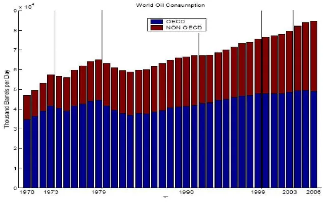
future oil supply shortfall is driving price of oil.

Figure 2: World oil consumption (yearly average)

According to the energy economics literature (Kim and Loungani (1992), Hamilton and

Herrera (2004)), oil price movements in 1973 and 1991 were caused by oil supply

disrup-tions during exogenous events in the Middle East (OPEC embargo and Iraq-Kuwait war,

respectively). However, as it is shown in Figure 2, yearly average world oil consumption was

increasing in the aftermath of 1991, while decreasing during the 1973-75 (OPEC embargo),

which means that supply cut argument is not valid for the 1991 oil price shock. Therefore,

Kilian(2009) claims that the latter is caused by the precautionary demand motive of the

firms using the oil as an input in their production. This motive is usually triggered by a

Middle East).

Based on this motivation, I build a theoretical model to quantify and examine the nature

of oil price shocks caused by precautionary demand in the crude oil market. Then I simulate

the effects of these demand shocks on the macroeconomic variables, such as GDP and

in-flation. In order to do that, I will construct a standard DSGE model with the sticky-prices

where firms can have access to an oil futures market. In this model, there is also the storage

operators, who buy the oil in the spot market and hedge it by selling the oil futures in the

futures market.

It is intuitive to think that in the case of an increased uncertainty about future oil supply,

the firms using oil as an input will buy futures and/or forwards contracts to guarantee a

future price and quantity. Moreover, higher demand in the futures market would encourage

the storage operators to increase their inventories and, thus, create scarcity in the spot

market for oil. That, in turn, will induce the spot price of oil to increase immediately.

This modification was first introduced by Alquist and Kilian (2010) to derive the immediate

effect of an uncertainty about the future oil supply shortfalls on the real spot price of oil.

They model the oil supply by a foreign country as an stochastic mean-preserving process.

When there is a news˝today about the future availability of the oil, the variance of the oil

endowment for tomorrow goes up permanently and creates an uncertainty shock. This setup

allows us to separate the mean effect (supply shock) from the variance effect (uncertainty

shock). Unlike Alquist and Kilian (2010) our model allows also for temporary increase in

an uncertainty in the market. However, if the concern of the agents are not realized (i.e. no

supply shortfall), they will reasonably update their beliefs and become less and less concerned

over time.

As another improvement on Alquist and Kilian (2010), we employ this extention in

a standard cashless DSGE model with the sticky-prices (Woodford (2003)) to analyze the

dynamics of macroeconomic variables when agitated by a future oil supply uncertainty. Since

oil is used as an input in the production process, any surge in its price, caused by a future

oil supply uncertainty or a current supply shortfall, will increase the production cost and

lead to a supply side˝ disturbance in the economy.

Recently, we became aware of related work by Unalmis, Unalmis and Unsal (2012).

They have independently studied the role of storage as a source of oil price shock and

examined its macroeconomic effects. Their setup is very similar to ours, however, they

introduce speculative demand shock only that ignores precautionary demand motives affected

by second-order through the volatlility in oil supply. Besides, unlike Unalmis, Unalmis and

Unsal (2012), our step is suitable to study monetary policy implications of oil prices shocks

in the presence of storage.

These findings also have important policy implications for thinking about the effects of

oil price changes on the U.S. economy. Some recent literature suggests that although high

oil prices contributed to recessions, they have never had a pivotal role in the creation of

those economic downturns (Bernanke et al. (1997), Leduc and Sill (1995)). In this regard,

As different oil price shocks causing different dynamics in income and inflation variation,

one has to consider the nature of the shock before any policy formuation to cope with those

adverse effects.

We find that under baseline Taylor-type interest rate rule, real oil price overshoots

to-gether with inflation and output loss and goes down below steady state at the next period

if uncertainties are not realized. However, if the shock is realized, i.e. followed by an actual

supply shock, the effect on inflation and output loss is high and persistent. In this case, the

existence of storage increases the variability of macroeconomic variables and real price of oil

by transmitting future worries into today’s decision making process.

The paper is organized as follows. Section 2 presents the model, Section 3 describes

competitive equilibrium, market clearing conditions and aggregation. Section 4 discusses

calibration and simulation results. Lastly, Section 5 concludes.

2

Literature Review

2.1

The Magnitude of the Oil Price Effect

Hamilton and Herrera (2004) and Hamilton (2005) point out that nine out of ten of the U.S.

recessions since World War II and every recession since 1973 were preceded by a spike in oil

prices. However, according to the Bureau of Economic Analysis and the Energy Information

Administration, between 1970 and 2005, residential and commercial and industrial energy

in oil prices can only explain a small fraction of the drop in GDP during a recession.

To solve this puzzle, Rotemberg and Woodford (1996) study output impulse response

functions and show that under imperfect competition the effect of oil price shock is stronger

under perfect competition. They estimate that a 1 percent innovation in energy prices lead

declines in U.S. output of 0.25 percent and in U.S. real wages of 0.09 percent about five to

six quarters later. Moreover, Finn (2000) shows that one can increase the response of an

oil price shock even under perfect competition when one models energy use as a function of

capacity utilization. She argues that an increase in the price of energy works as an adverse

technology shock to induce a contraction in the economics activity and the magnitude of

the force exerted by energy price shock derives from relationship between energy usage and

capital services.

However, both papers are silent on the business cycle properties of the model in response

to energy shocks. Precisely, they do not report the share of output fluctuations explained

by energy price shocks and the other business cycle facts such as volatility of investment,

consumption and co-movement of these variables. In fact, by incorporating energy use

exclu-sively on the production side in DSGE models, Kim and Loungani (1992) claim that energy

price fluctuations can only generate a small fraction of the output fluctuations observed in

U.S. data. They even conclude that all previous recessions would have occurred even without

energy shocks, since output is mainly driven by shocks to total factor productivity.

Besides, Dhawan and Jeske (2006) argue that introducing durable goods and household

volatil-ity, despite increasing total energy consumption in the economy. They find that household

with two different investment decision (durable and fixed capital) decrease their fixed capital

less than the stock of durables to balance their portfolio in response to an exogenous shock

(TFP or energy). This leads to fixed capital drop less than in a Kim and Loungiani type

economy and therefore explains why energy accounts for less output fluctuations in their

model. To solve the controversy of low share in total expenditure, high share in output

fluctuations, some studies claim that jump in energy prices make a substantial fraction of

the capital stock obsolete.

Bailey (1981) argues that as a result of high energy prices, energy inefficient machines

are shut down, and expected profits of machines in operation declines. The value of existing

capital decreases as it is not technologically suited to new economic conditions. Besides,

firms will not be willing to invest in new machines, unless the high prices period last for a

long time. Therefore, this mechanism will lead to low level of stock market prices. Although

this link was pronounced in the literature, only Wei (2003) analyzes the causal link between

energy price shock and stock marker crush in a equilibrium setup. In a

partial-equilibrium putty-model, where the real wage and interest rates are fixed exogenously, she

finds that an 80-percent permanent increase in the real energy price leads to a 10-percent

decline in the market value of previously installed machines. This impact is even smaller

(only 2-pecent decline) in a general-equilibrium putty-clay model, which is extreme case of

rigidity in the adjustment of capital ex post. According to Wei (2003), the energy price

large enough to offset most of the increase in cost coming from capital side.

The intuition for the decline in real wages is that with ex post Leontief technology, labor

cannot be reallocated to relatively efficient machines, which in turn reduces labor demand.On

the labor side, we should observe lower consumption and lower leisure as the high energy

prices generate wealth effect on the consumption behavior of the households. Lastly, the

real wage has to decline to clear the labor market. Lastly, some authors have argue that

stagflation of the 1970s were largely due to factors other than oil. Barsky and Kilian (2002)

claim that stagflation may have been partly caused by exogenous changes in monetary policy,

which coincided in time with the rise in oil prices. Bernanke, Gertler and Watson (1997)

argue that much of the decline in output and employment was due to the rise in interest

rates, resulting from the Feds endogenous response to the higher inflation induced by oil

shocks.

2.2

What has changed lately?

Blanchard and Gali (2007) define an oil shock as an episode where the overall increase in oil

price has been of more than 50% and has lasted for more than one year. Following this criteria

four oil shocks are identified for the period 1970-2005. Despite the fact that these oil shocks

are similar in magnitude, they have been associated with very different macroeconomic

performances. While the first two episodes (1973:2-1974:1 and 1978:4-1980:2) of oil price

increase coincide with an increase in all inflation variables and a decrease in GDP growth

GDP growth rate, an increasing real wage and low inflation. In the light of these evidences,

Blanchard and Gali (2007) try to explain the difference between various oil shocks assuming

that the source of the change in oil price is always the same, i.e. an exogenous increase in

oil price. They consider differences in monetary policy, in the degree of wage rigidity and

in the proportion of oil used in the production and show that a change in each of them can

reduce the volatility of both prices and quantities in response to the same oil shock.

However, Kilian (2009), Yucel, Brown, Nathan(??) and Campolini (2007) challenge the

idea that oil price shocks were alike, i.e. exogenous. They underline the importance of

identifying supply vs. demand shocks to oil prices. Campolini (2007) and Yucel,Brown,

Nathan(??) formulate the oil price shocks of 2000s as a persistent increase in foreign

pro-ductivity, while in 70s there was, simply, a reduction in oil supply. It is intuitive to expect

different sources of oil price increase to convey different dynamics. Namely, an exogenous

reduction in the supply of oil followed by high oil prices will boost marginal costs and

there-fore deliver an increase in inflation. This scenario is consistent with the observed data of

70s, but cannot be applied to 2000s. An exogenous and persistent increase in productivity of

foreign country (such as China) in a simple two-country model leads to an increase in foreign

GDP. Given the increased production, a persistent shock will induce a higher oil demand

and therefore drive the oil price up. The home economy will still experience higher oil prices

because of reduction in oil supply. However, there will be a reduction in the price of the

imported goods, as the foreign country is more productive now.As a result, CPI inflation in

wages.

Lastly, richer foreign country will buy more home-produced goods, and therefore output

in home country will also increase. Apparently, this story tells us that dynamics of oil price,

inflation, real wages and GDP observed in 2000s is consistent with an increase in oil demand

driven by an increase in productivity in countries like China and India.

On the other hand, Kilian (2010) takes this analysis further and claims that there is even

third type of oil price shock. He provides a decomposition of real oil price into oil supply

shock, shocks to the aggregate global demand for industrial commodities and demand shocks

that are specific to the oil market (i.e. precautionary oil demand). Using this decomposition,

he claims that, while the oil price increase in 70s is mainly due to precautionary demand

increase, in the current increase a crucial role is played by aggregate demand shocks.

3

The Model

This study extends the standard cashless Dynamic New Keynesian model as in Woodford

(2003) by adding an oil market. The are two countries in this model: an oil-importer and an

oil-exporter. The oil-importing country uses oil as an input in the production of intermediate

goods. Oil is supplied by the oil-exporting country, who recieves a random endowment in

each period. The oil-exporting country uses oil income to purchase the final good produced

3.1

The Oil-Importing Country

The oil-importing country consists of households, intermediate good producers, final good

producers and storage operators. Oil is used in the production of intermediate goods, which

are produced in a monopolistically competitive market. Oil is sold both at the spot and the

futures market.

3.1.1 The Final Good Sector

Final good is produced under perfect competition using continuum of differentiated

inter-mediate goods as inputs. The technology is defined by Dixit-Stiglitz aggregation formula,

Qt=

h Z 1

0

Qt(i)

ε−1

ε di

i ε ε−1

(1)

Profit-maximization and zero-profit condition for these firms implies that the demand for

intermediate good Qt(i) and the aggregate price level Pt are

Qt(i) =

h_Pt(i)

Pt

i−ε

Qt (2)

Pt =

h Z 1

0

Pt(i)1 −ε _dii

1 1−ε

3.1.2 The Intermediate Good Sector

There is a continuum of firms producing different varieties of intermediate goods under

mo-nopolistic competition. These firms have monopoly power over their output prices, however,

they compete for inputs on competitive factor markets. Therefore, they act as price takers on

factor markets, including the oil market. Besides, since these firms are very small, they take

aggregate variables as given. The production function for an intermediate good producer

type of itakes the following Cobb-Douglas form:

Qt(i) =AtKt(i)αkLt(i)αlOt(i)αo (4)

Intermediate good producers are exposed to a common techonological shock, At, which

evolves exogenously according to at = ηaat−₁ +ξ_a,t, where a_t ≡ logA_t and ξ_a,t is a white

noise with zero mean and σ2

a variance.

Price Setting

Intermediate good producers operate in a monopolistically competitive market. I follow the

literature on sticky-price models (Calvo(1983), Yun(1996)) and assume that although the

firms have monopoly power over their own prices, they reset their prices only infrequently.

At timet, only 1−θ fraction of firms adjust their prices. The rest of the firms cannot adjust

their prices and therefore set Pt(i) = Pt−₁(i).

A firm will maximize the expected discounted flow of future profits, if it gets a chance to

maxP˜t(i)Et Σ

∞

k=0(θ)kΛt,t+k[ ˜Pt(i)Qt+k(i)−Pt+kmct+kQt+k(i)]

subject to downward-sloping demand function

Qt+k(i) =

_P˜

t(i)

Pt+k

−ε

Qt+k

where Qt+k(i) is the demand for output produced by the firm i, and Λt,t+k is the discount

factor for the future nominal profits.

Futures Market:

Intermediate good producers also have an access to the financial markets. In order to avoid

uncertainty about future supply and about the price of oil, they buy futures contracts (Xt)

supplied by storage operators1_{. As I discuss in next section, there is no delivery in the futures}

market. Firms incur a profit (lost), if the price for futures fixed att to be delivered at t+ 1

is less (higher) than the spot price of oil at t+ 1. The intermediate firm’s problem in the

futures market is:

max

Xt

E0Σ

∞ t=0(

1 1 +rt

)thP

o t+1

Pt+1

− Ft

Pt+1

i

Xt

1

I state two different maximization problem for intermediate good producers: goods market and futures

market. However, one may suggest to combine these problems. In other words, in addition to factor inputs,

in each period firms can simultaneously choose the fraction of futures to be delivered, instead of settled by

cash payment. In this case, firms will buy oil from the spot market if they need any in excess of the futures

contracts provide them. However, I found out that the governing equations for this problem are the same

3.1.3 Storage Operators

Storage operators buy oil at spot market to fill their inventories. I assume that the storage

operators are risk-neutral, so all inventory is hedged by taking a long position in the oil

futures market. This implies that at time t the storage operator promises to sell a certain

amount of oil for Ft at time t+ 1. However, in the model there is no delivery, but only cash

settlement. The operator sells all the inventory carried from previous period at the spot

market (Po

tIt), settles the cash payments with the futures contract holders ((Ft−₁ −P_to)It),

and chooses the amount of inventory for the next period (It+1). Besides, following the

commodity pricing literature (Brennan (1991), Pyndick (1994, 2001)), we introduce the

convenience yield, g(It, σ2), which refers to the flow of benefits to the inventory holders.

These benefits arise from the fact that in the case of supply disruptions, the inventories can

help to satisfy the demand in the market and smooth the production process. Therefore, the

convenience yield is increasing in the level of inventories (g1(It, σt2)>0)2, but the marginal

convenience yield of an additional inventory is decreasing (g11(It, σ2t) < 0). Additionally,

since higher uncertainty about the future oil supply (high σ2

t) is more like to cause scarcity

in the market, the marginal convenience yield is increasing (g12(It, σt2) > 0) in σ2t. Lastly,

in order to ensure that the level of inventories is always positive, we assume that Inada

condition limIt→0 g1(It, σt2) =∞ holds. The optimization problem for the storage operator

2

We denotegias the derivative of gwith respect toithterm, wheregij implies cross-sectional derivative

is:

max

It+1

E0Σ

∞ t=0(

1 1 +rt

)thFt−1

Pt

It− P

o t

Pt

It+1+gt(It+1, σt+1)

i

(5)

The first-order condition for this problem yields the no-arbitrage condition for the storage

market:

Et

h ₁

1 +rt

Ft

Pt+1

i

= P

o t

Pt

−g₁(I_t+1, σ_t+1) (6)

3.1.4 Households

A representative household in the oil-importing country maximizes the following utility

func-tion:

E0 Σ

∞ t=0β

th

logCt− L

1+ψ t

1 +ψ

i

(7)

Households earn labor income wtPtLt, invest in risk-free bonds Bt+1, collect rent rktPtK¯t

from intermediate good producers and dividends Πtf for their ownership in the firms.3

PtCt+Bt+1 =Rt−₁Bt+wtPtLt+PtrktK¯t+ Πtf (8)

Maximizing the utility function with respect to Ct, Bt and Lt will give us the following

3

first-order conditions:

CtLtψ =wt (9)

1

Ct

=βEt

h ₁

Ct+1

RtPt

Pt+1

i

(10)

Equation(9) and (10) jointly characterizes the household’s decision rules for consumption,

labor supply and bond holding.

3.2

Monetary Policy

We assume that the monetary authority in the oil-importing country follows a standard

Taylor-type interest rate rule is similar to the one estimated by Clarida, Gali and Gertler

(2000) to characterize the historical U.S. monetary policy. This policy sets the nominal

interest rate for the risk-free bond to adjust output-inflation gap.

ˆ

Rt−φRRˆt−₁ = (1−φ_R)φ_ππ_t+ (1−φ_R)φ_yyˆ_t (11)

where ˆRtis the log deviation from steady-state nominal interest rate level ( ¯R),πt= logPt/Pt−₁

and ˆytis the log deviation of value-added from its steady state value. Since there is no

cross-border borrowing, the value-added (GDP) in the oil-importing country will be

3.3

Oil-Exporting Country

The oil-exporting country is modelled as an endowment economy and acts as a price-taker in

the spot market for oil. In each period, it receives a random oil endowment Ωt. Oil revenues

are used to buy consumption good produced in the oil-importing country.

In each period, the oil-exporting country acts as a price-taker in spot market for oil and uses

revenues to buy consumption goods from final good procuders.

PtCtF =PtoΩt (13)

In order to disentangle news shock˝ from the mean shock, I assume that the percentage

deviation of the stochastic oil endowment from its steady state ( ˆωt ≡ ln(Ωt)−ln( ¯Ω)) has

the following property:

ˆ

ωt+1 =ρωˆt+ ξt+1 (14)

ξt+1 =utεt+1 (15)

ut=λut−₁+σuηt (16)

To be more concise, if there is no news˝, (ηt = 0), or in other words no uncertainty about

the future availability of the oil supply, the oil endowment will be at steady-state level. On

the other hand, if there is anews shock˝at time t (ηt>0), the variance of the ˆωt+1 will be

positive. However, this does not neccesarily imply that the supply will be less at t+ 1, since

4

Equilibrium, Market Clearing and Aggregation

4.1

Sticky-price Equilibrium

We assume a symmetric monopolistic competition equilibrium in which all intermediate good

producing firms have identical behavior. In this equilibrium, at a given time some of the

intermediate good producing firms cannot adjust their prices. However, those firms that

optimize their profits, decide to charge the same price ˜Pt. Therefore, the aggregate price

index will be:

Pt= [(1−θ) ˜Pt

1−ε

+θP1−ε t−₁]

1

1₋ε (17)

If we denote ˜pt=

˜

Pt

Pt, then

˜

pt =

h₁−θπ¯_tε−1

1−θ i 1

1−ε

(18)

4.2

Aggregation

Aggregate price dispersion has a distortionary effect on the aggregate output. If we denote

aggregate price dispersion by ∆t=

R1 0(

Pt(i)

Pt )

−ε_{di, aggregate output will be the following:}

Qt =

AtKtαkLαtlO αo

t

∆t

(19)

Lt=

Z 1 0

Lt(i)di (20)

Kt=

Z 1 0

Kt(i)di (21)

Ot=

Z 1 0

Ot(i)di (22)

In the production factors market, monopolistic distortion caused by the intermediate

good producing firms implies that labor, capital and oil are paid below their marginal

prod-uct.

wtLt=αlmctQt∆t (23)

rktKt=αkmctQt∆t (24)

potOt=αomctQt∆t (25)

where real marginal cost mct= po

tαowtαlrktαk

Atαoαoαlαlαkαk is common for all firms. Under flexible prices,

monopoly distortion measured bymctis constant and less than unity. However, when prices

are sticky, it responds to the real and nominal shocks in the economy. Therefore, an oil price

shock affects the inputs market through the pertubation in mct.

Optimal price-setting decision ( ˜Pt) by an intermediate good producing firm is governed

by the following equations:

˜

Pt

Pt

≡p˜_t =

EtΣ∞k=0(βθ)k Qt

+k

Ct+kX

−ε t,k

ε

ε−₁mct+k

EtΣ∞k=0(βθ)k Q

t+k

Ct+kX

1−ε t,k

≡ Nt

Dt

(26)

Nt =

ε ε−1mct

Qt

Ct

+βθEtπ¯tε+1Nt+1 (27)

Decision rules for the intermediate firms and the storage operators in the financial

mar-kets, which determine the equilibrium level of oil inventories and futures contracts, are

characterized by the following equations:

Et (pot+1) = Et (

Ft

Pt+1

) (29)

Et

h ₁

1 +rt

Ft

Pt+1

i

=po

t −g1(It+1, σ2t+1) (30)

4.3

Market Clearing

In equilibrium, net supply of riskless bonds should be zero. Besides, since there is no capital

accumulation, aggregate demand for capital is equal to the fixed supply.

Bt= 0 (31)

Kt= 1 (32)

In the oil market, oil supply is determined by the stochastic endowment (Ωt) and the

change in the level of inventories (∆It+1). Therefore, the aggregate demand for oil, Ot, is

equal to Ωt−∆I_t+1.

The oil-exporting country spends all the oil revenues on consumption good produced by

the final good producers in the oil-importing country. Therefore, in the equilibrium, goods

market clearing implies:

CtF =p o

tOt (33)

5

Calibration and Results

We follow the literature to calibrate the parameters for the utility and production functions.

We set β = 0.99 corresponding to %4 annual steady-state real interest rate. Utility is

logarithmic and the parameter ψ = 1 implying unit Frisch labot elasticity. There is no

capital accumulation in the model, so the aggregate level of capital, ¯K, is set to 1. The

labor, capital and oil elasticities of gross output are set to 0.63, 0.32 and 0.05, respectively.

The elasticity of substition among intermediate goods, ε, is set to 7.66 to match a

steady-state price mark-up of %15 implying µ = 1.15. Together with the oil elasticity of gross

output, αo = 0.05, the price mark-up matches the average oil consumption share of U.S.

GDP, which is 0.04. We assume that the intermediate firms can optimize their profits only

once a year, so the Calvo price adjustment parameter, θ, is set to 0.75.

For the baseline analysis, we calibrate the monetary policy using the findings Orphanides

(2001). Therefore, we set our baseline parameters to φR = 0.79, φπ = 1.8 and φy = 0.27.

We will later simulate the model using alternative policies by changing the coefficients of the

interest rate smoothing parameter and the coefficients of the contemporaneous inflation and

the log-deviation of the output.

The persistence parameters for the technology (η), oil endowment (ρ) and the variance

(λ) shocks are all set to 0.5. The calibration of these parameters do not have any significant

qualitative effect on the results, as long as they are set positive numbers less than one.

Following (Gorton et al. (2007)), we set the marginal convenience yield parameters for

endowment and the inventory are chosen to be 0.5 and 0.05.

We solve the model by taking second-order Taylor expansion around deterministic

steady-state with zero inflation in order to capture the variance effect and calculate impulse response

functions for the specific shocks. To be more precise, the solution method follows the

al-gorithm proposed by Benigno, Benigno and Nistico (2010), which proposes a second-order

appproximation method for the solution of the dynamic stochastic models, where exogenous

state variables display time-varying risk.

5.1

Precautionary Demand Shock

We model precautionary demand shock as anews shock˝to the variance of oil endowment.

Once there is a shock to the σt+1, firms become worried about the future availability of the

oil supply and demand more futures contracts to offset that uncertainty. On the other hand,

the storage operators increase their inventories to sell more futures contracts. In order to

show formally how the uncertainty about future oil supply may increase the real spot price

oil, we solve the maximization problem for the storage operators and the intermediate good

producing firms, and aggregate production to get the following equation:

mctQ ′

(Ωt−∆It+1)

| {z }

po,t

=Et[

1 1 +rt

mct+1Q

′

(Ωt+1−∆I_t+2)

| {z }

po,t+1

] +g1(It+1, σt+1) (35)

When there is a “news shock”at time t, not followed by any change in the mean at time

is disturbed upward by Jensen inequality as Q′

(·) is convex. In order to offset that wedge,

the level of inventory holdings decided to hold at time t to be used at time t + 1, It+1,

will increase to raise the left-hand side through ∆It+1 and lower the right-hand side of the

equation through ∆It+2 and g1(·). Meantime, we will observe a spike in the real spot price

of oil, po,t, since it is equal to mctQ′(Ωt−∆I_t+1).

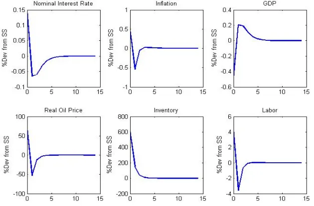
Figure 3: Shock to the variance (ηt= 1), no realization (εt = 0 for allt)

We simulate the model with the benchmark Taylor-rule estimated by Orphanides (2001)

using real-time data for 1979:1995. Figure 3 shows the dynamics of inflation, percentage

deviation of GDP, inventory, real oil price and interest rates from their steady state values

responding one standard deviation in σt+1.

In accordance with the model, changes in inflation, inventories and oil price are positive

output) during the second period, since oil supply shortfall does not occur. The level of oil

inventories do not go back to the steady-state level immediately, since there is still concern,

although less, about t+ 2. Besides, the amount of oil in the economy, Ω−∆I_t+2 is higher

than its steady state value, so the spot price of oil and inflation are below and output above

their steady-state values. Oil abundance lasts as long as the uncertainty is not vanished and

oil supply shortfall does not occur.

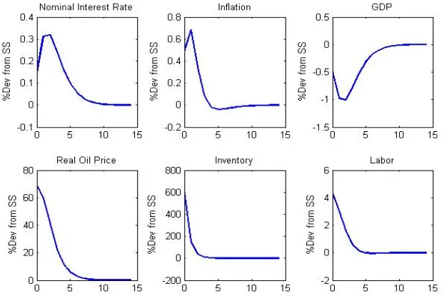
Figure 4: Shock to the variance (ηt= 1) followed by a shock to the mean (εt+1 =−1)

The difference can be seen in Figure 4, where an uncertainty shock at timetis followed by

a supply shock at timet+ 1. Since there is no more oil abundance in the economy during the

6

Conclusion

In this study we model and quantify the effect of uncertainty about future availability of oil

supply on the macroeconomy. Our setup allows us to separate mean effect (supply shock)

from variance shock (uncertainty effect). Under baseline Taylor-type interest rate rule, real

oil price overshoots (and perturbates inflation and output loss) and goes down below steady

state at the next period if uncertainties are not realized. However, if this shock is realized,

i.e. followed by an actual supply shock, the effect on inflation and output loss is high and

7

Reference

Barsky, R. and Killian L., (2002), Do We Really Know that Oil Caused the Great

Stagfla-tion? A Monetary Alternative˝, NBER Macroeconomics Annual 2001, 137-183.

Benigno, G., Benigno, P., and Nistico S., (2010), Second-Order Approximation of

Dy-namic Models with Time-Varying Risk˝,NBER Working Paper Series, 16633.

Benigno, P. and Woodford M. (2004), Optimal Monetary and Fiscal Policy: A Linear

Quadratic Approach˝, NBER Working Papers, 9905.

Bernanke, B.S., Gertler M., and Watson M., (1997), Systematic Monetary Policy and the

Effects of Oil Price Shocks˝, Brookings papers on Economic Activity,1, 91-157.

Blanchard, Olivier J., and Gali J., (2007a) Real Wage Rigidities and the New

Keyne-sian Model˝,Journal of Money, Credit and Banking, 39, 3565. Blanchard, J.O. and Gali J.,

(2007b), The Macroeconomic Effects of Oil Shocks: Why Are the 2000s So Different from

70s˝, NBER Working paper, 13368.

Carlstrom, C.T. and Fuerst T.S., (2006), Oil Prices, Monetary Policy, and

Campolmi, A., (2009), Oil Price Shocks: Demand vs Supply in a Two-Country Model˝,

mimeo.

Calvo, G.A., (1983), Staggered Prices in a Utility-maximizing Framework˝, Journal of

Monetary Economics, 12(3), 383-39.

Clarida, R., Gali, J., and Gertler, M. (2000), Monetary Policy Rules and Macroeconomic

Stability: Evidence and Some Theory˝The Quarterly Journal of Economics, 115(1), 147-180.

Dhawan, R. and Jeske K., (2006), Energy Price Shocks and the Macroeconomy: The Role

of Consumer Durables˝, Federal Reserve Bank of Atlanta, Working papers.

Frankel, J. (2008),The Effect of Monetary Policy on Real Commodity Prices˝inAsset Prices

and Monetary Policy, John Campbell, ed., U.Chicago Press, 291-327

Gorton G.B., Hayashi F. and Rouwenhorst K.G., (2007), The Fundamentals of Commodity

Futures Returns˝, NBER Working paper, 13249.

Hamilton, J. and Herrera A.M., (2004), The Oil Shocks and Aggregate Macroeconomic

Behavior: The Role of Monetary Policy˝, Journal of Money, Credit, and Banking, 36,

Khan, A., King, R.G. and Wolman, A. L., (2003), Optimal Monetary Policy˝, Review

of Economic Studies 70, 825860.

Kilian, L., (2009), Not All Oil Price Shocks Are Alike: Disentangling Demand and Supply

Shocks in the Crude Oil Market˝,American Economic Review, 99(3), 1053-1069.

Kilian, L. and Alquist R., (2010), What do we learn from the price of crude oil futures?˝,

Journal of Applied Econometrics, 25(4), 539-573.

Kim, I. and Loungani P., (1992), The Role of Energy in Real Business Cycle Models˝,

Journal of Monetary Economics, 29(2), 173-189.

Leduc, S. and Sill K., (2004), A Quantitative Analysis of Oil Price Shocks, Systematic

Monetary Policy, and Economic Downturns˝, Journal of Monetary Economics, 51(4),

781-808.

Rotemberg, J.J., and Woodford M., (1996), Imperfect Competition and the Effects of

En-ergy Price Increase on Economic Activity˝, Journal of Money, Credit, and Banking, 28(4),

Schmitt-Grohe, S., Uribe, M. (2004a). Optimal Operational Monetary Policy in the

Christiano-Eichenbaum-Evans Model of the U.S. Business Cycl etextacutedbl, NBER Working Papers,

10724

Unalmis, D., Unalmis, I. and Unsal D.F., (2012) On the Sources and Consequences of

Oil Price Shocks: the Role of Storage˝,Working paper. Wei, C., (2003),The Stock Market,

and the Putty-Clay Investment Model˝, American Economic Review, 93(1), 311-323.

Woodford, M. (2003), Interest and Prices: Foundations of a Theory of Monetary Policy,

Princeton: Princeton University Press.

Yun, T., (1996),Nominal Price rigidity, Money Supply Endogeneity, and Business Cycles˝,