http://www.scirp.org/journal/am ISSN Online: 2152-7393
ISSN Print: 2152-7385
Verification of Real-Time Pricing Systems Based
on Probabilistic Boolean Networks
Koichi Kobayashi
1*, Kunihiko Hiraishi
21Graduate School of Information Science and Technology, Hokkaido University, Sapporo, Japan 2School of Information Science, Japan Advanced Institute of Science and Technology, Ishikawa, Japan
Abstract
In this paper, verification of real-time pricing systems of electricity is considered us-ing a probabilistic Boolean network (PBN). In real-time pricus-ing systems, electricity conservation is achieved by manipulating the electricity price at each time. A PBN is widely used as a model of complex systems, and is appropriate as a model of real- time pricing systems. Using the PBN-based model, real-time pricing systems can be quantitatively analyzed. In this paper, we propose a verification method of real-time pricing systems using the PBN-based model and the probabilistic model checker PRISM. First, the PBN-based model is derived. Next, the reachability problem, which is one of the typical verification problems, is formulated, and a solution method is derived. Finally, the effectiveness of the proposed method is presented by a numeri-cal example.
Keywords
Model Checking, Probabilistic Boolean Networks, Real-Time Pricing
1. Introduction
In recent years, there has been growing interest in energy and the environment. For problems on energy and the environment such as energy saving, several approaches have been studied (see, e.g., [1][2]). In this paper, we focus on real-time pricing sys-tems of electricity. A real-time pricing system of electricity is a system that charges dif-ferent electricity prices for difdif-ferent hours of the day and for difdif-ferent days, and is ef-fective for reducing the peak and flattening the load curve (see, e.g., [3]-[6]). In general, a real-time pricing system consists of one controller deciding the price at each time and multiple electric consumers such as commercial facilities and homes. If electricity con-servation is needed, then the price is set to a high value. Since the economic load be-How to cite this paper: Kobayashi, K. and
Hiraishi, K. (2016) Verification of Real-Time Pricing Systems Based on Probabilistic Boo-lean Networks. Applied Mathematics, 7, 1734- 1747.
http://dx.doi.org/10.4236/am.2016.715146
Received: July 26, 2016 Accepted: September 13, 2016 Published: September 16, 2016 Copyright © 2016 by authors and Scientific Research Publishing Inc. This work is licensed under the Creative Commons Attribution International License (CC BY 4.0).
http://creativecommons.org/licenses/by/4.0/
1735
comes high, consumers conserve electricity. Thus, electricity conservation is achieved. In the existing methods, the price at each time is given by a simple function with respect to power consumptions and voltage deviations and so on (see, e.g., [6]). In order to realize more precisely pricing, it is necessary to use a mathematical model of consumers.
On the other hand, in order to deal with complex systems such as power systems and gene regulatory networks, it is one of the appropriate methods to approximate a com-plex system by a discrete abstract model (see, e.g., [7]). In addition, human decision making is also complex, and is modeled by a discrete model (see, e.g., [8]). Thus, in analysis and control of complex systems and those with human decision making, a dis-crete model plays an important role. Several disdis-crete models have been proposed so far (see, e.g., [9]). In this paper, we focus on a Boolean network (BN) [10]. In a BN, the state is given by a binary value (0 or 1), and the dynamics are expressed by a set of Boo-lean functions. Since BooBoo-lean functions are used, it is easy to understand the interaction between states. In addition, the behavior of complex systems is frequently stochastic by the effects of noise. From this viewpoint, a probabilistic BN (PBN) has been proposed in [11]. In a PBN, a Boolean function is randomly decided at each time among the can-didates of Boolean functions.
Under the above backgrounds, the authors have proposed in [12] the PBN-based model of real-time pricing systems. In this model, decision making of electric consum-ers is modeled by a PBN. That is, decisions of a consumer are modeled by Boolean functions, and one of decisions is selected probabilistically. Selection probabilities are controlled by the price at each time. In [12], an approximate algorithm for solving the optimal control problem has been proposed. However, analysis and verification using the PBN-based model have not been considered.
In this paper, we propose a verification method of real-time pricing systems using the PBN-based model and the probabilistic model checker PRISM [13]. Using PRISM, we can verify whether this system satisfies the specification described by probabilistic computation tree logic (PCTL) [14] or not. The reachability problem is considered as one of the typical verification problems, and a numerical example is presented. The proposed method provides us a basic of model-based design of real-time pricing systems.
In Section 2, the outline of real-time pricing systems studied in this paper is ex-plained. In Section 3, the PBN-based model is exex-plained. In Section 4, the verification problem is formulated. In Section 5, a solution method using PRISM is proposed. In Section 6, a numerical example is presented. In Section 7, we conclude this paper.
Notation: For the n-dimensional vector x
[
x x1 2 xn]
Τ
= and the index set
{
i i1, ,2 ,im} {
1, 2, ,n}
= ⊆
,
[ ]
xi i : xi1 xi2 ximΤ
∈ = is defined.
2 Real-Time Pricing Systems
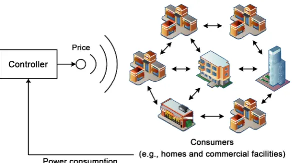
In this section, we explain the outline of real-time pricing systems studied in this paper.
Figure 1. Illustration of real-time pricing systems.
monitor the status of electricity conservation of other consumers. In other words, the status of some consumer affects that of other consumers. For example, in commercial facilities, we suppose that the status of rival commercial facilities can be checked by lighting, Blog, Twitter, and so on. Depending on power consumption, i.e., the status of electricity conservation, the controller determines the price at each time. If electricity conservation is needed, then the price is set to a high value. Since the economic load becomes high, consumers conserve electricity. Thus, electricity conservation is achieved. The price does not depend on each consumer, and is uniquely determined.
In this paper, decision making of electric consumers is modeled by a probabilistic Boolean network (PBN). Here, we suppose that each electric consumer has candidates of a decision in electricity conservation, and one of candidates is selected probabilisti-cally depending on the electricity price at the current time. In such a case, it is appro-priate to adopt the PBN-based model. In this paper, the property of real-time pricing systems can be verified using the PBN-based model.
3. Modeling Using Probabilistic Boolean Networks
In this section, first, we explain the outline of PBNs. Next, each consumer in real-time pricing systems is modeled by a PBN.
3.1. Probabilistic Boolean Networks
First, we explain a (deterministic) Boolean network (BN). A BN is defined by
(
)
( )( )
( )
(
)
(
)
( )( )
( )
(
)
(
)
( )( )
( )
(
)
1
2
1 1
2 2
1 ),
1 ,
1 n ,
j j
j j
n
n j j
x k f x k
x k f x k
x k f x k
∈
∈
∈
+ =
+ =
+ =
(1)
where :
[
1 2]
{ }
0,1n n
1737
{ }
( ){ }
1: 0,1 0,1
i
i
f → is a given Boolean function consisting of logical operators such as AND (∧), OR (∨), and NOT (¬). If ( )i = ∅
holds, then x ki
(
+1)
is uniquely determined as 0 or 1.Next, we explain a probabilistic Boolean network (PBN) (see [11] for further details). In a PBN, the candidates of ( )i
f are given, and for each xi, selecting one Boolean function is probabilistically independent at each time. Let
( )
( )
( )
(
i)
, 1, 2, ,( )
l i
l j j
f x k l q i
∈
=
denote the candidates of ( )i
f . The probability that fl( )i is selected is defined by ( )i : Prob
(
( )i ( )i)
.l l
c = f = f
Then, the following relation
( ) ( ) 1 1 q i i l l c = =
∑
(2)
must be satisfied. Probabilistic distributions are derived from experimental results. Fi-nally, i, i=1, 2,,n are defined by
( ) ( ) 1 : . q i i i l l= =
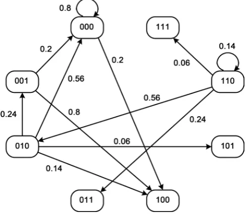
We show a simple example.
Example 1. Consider the PBN in which Boolean functions and probabilities are giv-en by
( ) ( )
( )
( )( )
( )
( )1 1
1 3 1
1
1 1
2 3 2
, 0.8,
, 0.2,
f x k c
f
f x k c
= =
=
= ¬ =
( )2 ( )2
( )
( )
( )21 1 3 , 1 1.0,
f = f =x k ∧ ¬x k c =
( ) ( )
( )
( )
( )( )
( )
( )3 3
1 1 2 1
3
3 3
2 2 2
, 0.7,
, 0.3,
f x k x k c
f
f x k c
= ∧ ¬ =
=
= =
where q
( )
1 =2, q( )
2 =1 and q( )
3 =2 hold, 1={ }
3 , 2 ={ }
1, 3 , and{ }
3= 1, 2
hold, and we see that the relation (2) is satisfied. Next, consider the state trajectory. Then, for x
( )
0 =[
0 0 0]
Τ, we can obtain( )
[
] ( ) [
]
(
)
Prob x 1 = 0 0 0 | Τ x 0 = 0 0 0Τ =0.8,
( )
[
] ( ) [
]
(
)
Prob x 1 = 1 0 0 | Τ x 0 = 0 0 0Τ =0.2.
In this example, the cardinality of the finite state set
{ }
30,1 is given by 23 =8, and we obtain the state transition diagram of Figure 2 by computing the transition from each state. In Figure 2, the number assigned to each node denotes x1, x2, x3
Figure 2. State transition diagram.
3.2. Model of Consumers
Consider modeling the set of consumers as a PBN. The number of consumers is given by n. We assume that the state of consumer i∈
{
1, 2,,n}
is binary, and is denoted byi
x . The state implies
0 consumer conserves electricity,
1 consumer normally uses electricity. i
i x
i
=
The binary value of xi is determined by power consumption of consumer i. In ad-dition, we assume that the probability ( )i
l
c is time-varying and is changed by the price at each time. That is, the probability is given by
( )i
( )
( )i ( )i( )
,l l l
c k =a +b u k
where
( )
1u k ∈ ⊂ is the price (the control input). We assume that the set is a finite set, and for any u∈ , two conditions (2) and 0≤cl( )i
( )
k ≤1 hold. The Boo-lean function ( )il
f must be derived depending on real situations and experimental re-sults. In this paper, as one of examples, we consider the following situation, which will mimic a real situation.
Let i⊆
{
1, 2,,n}
, i=1, 2,,n denote the set of consumers, which affect to con-sumer i. We assume that there exists one leader in the local area. The state of a leader is given by x1. Then, for consumer i, we consider the following model Σi:(
)
( ) ( )
( )
( ) ( )( )
( ) ( )
( )
( ) ( )( )
( )
( )
( )( )
( ) ( )( )
( ) ( )
(
( )
)
( ) ( ) ( )( )
( )
( )
( )( )
( ) ( )( )
1 1 1 1
2 2 2 2
3 3 3 3
4 4 4 4
5 1 5 5 5
1, ,
0, ,
, ,
1
, ( ) ,
, ,
i
i i i i
i i i i
i i i i
i i
i i i i i
j j
i i i i
f c k a b u k
f c k a b u k
f x k c k a b u k
x k
f g x k c k a b u k
f x k c k a b u k
∈
= = +
= = +
= = +
+ =
= = +
= = +
1739
The Boolean functions 1( )
i
f and 2( )
i
f imply that consumer i forcibly conserves (or does not conserve) electricity. In these cases, time evolution of the state does not de-pend on the past state. The Boolean function 3( )
i
f implies that the state is not changed. The Boolean function 4( )
i
f implies that the state of consumer i is changed depending on the other consumers. The Boolean function 5( )
i
f implies that the state of consumer
i is changed depending on the leader. Thus, decision making of consumers can be modeled by a PBN. Of course, we may use other Boolean functions.
4. Problem Formulation
In this section, the verification problem described by probabilistic computation tree logic (PCTL) is formulated for the PBN-based model of consumers (see Appendix A for details on PCTL).
Here, the reachability problem is formulated as one of the typical problems. For the system Σi, i=1, 2,,n given by (3), the output
( )
1( ) ( )
2( )
{ }
0,1 p py k =y k y k y k Τ∈ is defined, where yi =xj, j∈
{
1, 2,,n}
. We remark that the output is not the measured signal. First, the reachability problem is given.Problem 1. Suppose that for the system Σi, i=1, 2,,n given by (3), the initial
state x
( )
0 =x0, the control time N, and the target output yf are given. Then, find amaximum probability p satisfying
( )
(
F N)
p y k yf
≤
≤ =
by manipulating a control input sequence u
( ) ( )
0 ,u 1 ,,u N(
−1)
.Let Pmax denote the maximum probability obtained by solving this problem. In this
problem, we find a maximum probability that y k
( )
= yf holds within time N. In the conventional reachability problem, only terminal time is focused, and it is checked whether y N( )
=yf holds or not. In this paper, we focus on not only terminal time N but also other times 0,1,,N−1. Since the system has the control input, we find a maximum probability satisfying the condition. In the case where peak demand is fo-cused on, y k( )
= yf may be replaced with y k( )
≤γ , where γ is a given constant.Furthermore, by solving Problem 1 at each time, a kind of model predictive control (MPC) can be realized (see Section 5.3 for further details).
5. Solution Method Using PRISM
In this section, we consider a solution method for Problem 1 using the probabilistic model checker PRISM [13].
5.1. Preparation: Transformation of Boolean Functions
As a preparation, the following lemma [15] is introduced.
Lemma 1. Consider two binary variables δ δ1, 2. Then the following relations hold.
i) ¬δ1 is equivalent to 1−δ1.
iii) δ δ1∧ 2 is equivalent to δ δ1 2.
For example, δ1∨ ¬δ2 is equivalently transformed into
(
)
(
)
1 1 2 1 1 2 1 2 1 2
δ + −δ −δ −δ = −δ +δ δ . By using this lemma, a Boolean function can be transformed into a polynomial with binary variables.
5.2. Description in PRISM
To solve Problem 1 and the verification problem described by PCTL formulas, the probabilistic model checker PRISM is used. PRISM supports a discrete-time Markov chain (DT-MC), a continuous-time Markov chain (CT-MC), and a Markov decision process (MDP). PRISM consists of three parts: “Model”, “Properties”, “Simulator”. In the “Model” part, a given probabilistic system is described using the PRISM language. In the “Properties” part, the property specification language incorporates temporal log-ic such as PCTL, and we can verify whether a given PCTL formula holds or not. In the “Simulator”, the state trajectories can be simulated.
Using PRISM, consider modeling the system Σi, i=1, 2,,n given by (3). To ex-plain the PRISM-based method, consider the following model of three consumers:
(
)
( ) ( )( )
( ) ( )( )
( )
( )( )
( )( )
( )
( )( )
( )
( )( )
( )
( )( )
( )( )
( )
1 1 1 1 1 1 2 2 1 11 3 1 3
1 1
4 2 3 4
1 1
5 1 5
1, 0.1,
0, 0.025 ,
1 , 0.9 0.1 ,
, 0.05 ,
, 0.025 ,
f c k
f c k u k
x k f x k c k u k
f x k x k c k u k
f x k c k u k
= = = = + = = = − = ∧ = = =
(
)
( ) ( )( )
( ) ( )( )
( )
( )( )
( )( )
( )
( )( )
( )
( )( )
( )
( )( )
( )( )
( )
2 2 1 1 2 2 2 2 2 22 3 1 3
2 2
4 1 3 4
2 2
5 1 5
1, 0.1,
0, 0.025 ,
1 , 0.9 0.1 ,
, 0.05 ,
, 0.025 ,
f c k
f c k u k
x k f x k c k u k
f x k x k c k u k
f x k c k u k
= = = = + = = = − = ∧ = = =
(
)
( ) ( )( )
( ) ( )( )
( )
( )( )
( )( )
( )
( )( )
( )( )
( )
( )( )
( )( )
( )
3 3 1 1 3 3 2 2 3 33 3 1 3
3 3
4 1 2 4
3 3
5 1 5
1, 0.1,
0, 0.025 ,
1 , 0.9 0.1 ,
( ), 0.05 ,
, 0.025 .
f c k
f c k u k
x k f x k c k u k
f x k x k c k u k
f x k c k u k
= = = = + = = = − = ∧ = = =
In addition, is given by =
{
3, 4, 5}
. Then, the PRISM source code describing this system is shown as follows.01: mdp
02: module RTP1 03: x1: [0..1] init 1;
1741
05: [RTP] u=4 -> 0.1:(x1’=1) + 0.1:(x1’=0) + 0.5:(x1’=x1) + 0.2:(x1’=x2*x3) + 0.1:(x1’=x1)
06: [RTP] u=5 -> 0.1:(x1’=1) + 0.125:(x1’=0) + 0.4:(x1’=x1) + 0.25:(x1’=x2*x3) + 0.125:(x1’=x1)
07: endmodule 08: module RTP2 09: x2:[0..1] init 1;
10: [RTP] u=3 -> 0.1:(x2’=1) + 0.075:(x2’=0) + 0.6:(x2’=x2) + 0.15:(x2’=x1*x3) + 0.075:(x2’=x1)
11: [RTP] u=4 -> 0.1:(x2’=1) + ... (omit) 12: [RTP] u=5 -> 0.1:(x2’=1) + ... (omit) 13: endmodule
14: module RTP3 15: x3:[0..1] init 1;
16: [RTP] u=3 -> 0.1:(x3’=1) + 0.075:(x3’=0) + 0.6:(x3’=x3) + 0.15:(x3’=x1*x2) + 0.075:(x3’=x1)
17: [RTP] u=4 -> 0.1:(x3’=1) + ... (omit) 18: [RTP] u=5 -> 0.1:(x3’=1) + ... (omit) 19: endmodule
20: module input 21: u:[3..5] init 3; 22: [RTP] u=3 -> (u’=3); 23: [RTP] u=3 -> (u’=4); 24: [RTP] u=3 -> (u’=5); 25: [RTP] u=4 -> (u’=3); 26: [RTP] u=4 -> (u’=4); 27: [RTP] u=4 -> (u’=5); 28: [RTP] u=5 -> (u’=3); 29: [RTP] u=5 -> (u’=4); 30: [RTP] u=5 -> (u’=5); 31: endmodule.
In line 1, it is described that a given system is an MDP, i.e., the control input (in oth-er words, the nondetoth-erministic variable) that must decide is included. In lines 2-7, the dynamics for x1 (consumer 1) are modeled. In line 3, it is described that x1 takes a
binary value, and the initial value of x1 is given by x1
( )
0 =1. In line 4, if u k( )
=3 holds, then the value of x1 at the next time is given by 1 with the probability 0.1, 0with the probability 0.075, x1 (i.e., the state is not changed) with the probability 0.6, 2 3
x x (corresponding to x2
( )
k ∧x3( )
k1) with the probability 0.15, and 1
x with the probability 0.15. Similarly, in line 5, the case of u k
( )
=4 is described. In line 6, the case of u k( )
=5 is described. In lines 8-13, the dynamics for x2 (consumer 2) are modeled. In lines 14-19, the dynamics for x3 (consumer 3) are modeled. In thissys-1In PRISM, given Boolean functions may be directly used (see http://www.prismmodelchecker.org/ for
tem, a discrete probabilistic distribution is given for each xi. Hence, in PRISM, the dynamics for each xi must be modeled separately. In lines 20-31, the property of the control input is described as a nondeterministic variable. We note here that the initial value of the control input must be given (see line 21). Finally, to associate with each module, [RTP] is described in lines 4-6, 10-12, 16-18, 22-30.
From the above example, we see that the system Σi, i=1, 2,,n given by (3) can be described by PRISM. Finally, we present a procedure for deriving the PRISM source code as follows. In the following procedure, without loss of generality, the input set is given by =
{
1, 2,,}
.Derivation Procedure of PRISM Source Code:
Step 1: Transform each Boolean function into a polynomial with binary variables by using Lemma 1. Let ˆ( )i
l
f denote the obtained polynomial. Step 2: Describe that a given system is an MDP.
Step 3: Compute the probability ( )i l
c for each element of . Let ( ),
i l p
c denote the probability for p∈.
Step 4: Describe module RTP i, i=1, 2,,n as follows. module RTP i;
i
x :
[ ]
0..1 init xi( )
0 ;[RTP] 1 1,1( ):
(
ˆ1( ))
5,1( ):(
ˆ5( ))
i i i i
i i
u= →c x′= f + + c x′= f ;
[RTP] ( )
(
( ))
( )(
( ))
1 5
1, : ˆ 5, : ˆ
i i i i
i i
u= →c x′= f + + c x′= f ; endmodule.
Step 5: Describe the control input u as follows. module input
u: 1.. init u
( )
0 ; [RTP] ui = →1(
ui′=1)
;
[RTP] ui= →1
(
ui′= )
; [RTP] ui= →
(
ui′=1)
; [RTP] ui= →
(
ui′= )
; endmodule.The above procedure is the improved version of the procedure proposed in [16].
5.3. Verification and Application to MPC
Several properties described by PCTL formulas can be verified by using the obtained model on PRISM. We use the “Properties” part in PRISM.
Consider solving Problem 1 (the reachability problem). Then, we use Pmax prepared
in PRISM. Suppose
[
]
T 1 2y= y y and yf =
[ ]
0 1T. Then in PRISM, this problem is described by(
) (
)
max ? F N 1 0 & 2 1 .
1743
This implies that find a maximum probability Pmax satisfying the following
condi-tion: at time k=0,1,,N, the number of times that y k
( )
=yf holds is greater than or equal to 1, i.e., this code expresses the reachability problem itself.From the above results, we see that the verification problem can be easily imple-mented by using PRISM. The control input sequence u
( ) ( )
0 ,u 1 ,,u N(
−1)
is ob-tained simultaneously, but in PRISM 4.0.3, the obob-tained control input sequence cannot be displayed except for the case of N= ∞. In the case of N= ∞, the discrete-time Markov chain can be obtained as the closed-loop system of a given system. The control input sequence can be obtained by exploratory analysis using the simulator in PRISM. Otherwise, this sequence can be obtained by solving the control problem such as the optimal control problem. In both cases, the verification result will be useful.On the other hand, the problem of finding Pmax and a control input sequence can
be regarded as a kind of the control problem. Noting that the initial value of the control input must be given, a kind of MPC can be realized by the following procedure.
[Procedure of MPC]
Step 1: Set t=0, and determine the current state x t
( )
=xt according to power consumption.Step 2: Find the current control input u∗
( )
t maximizing Pmax. That is, for each( )
u t ∈ , solve Problem 1.
Step 3: Apply only the control input at t, i.e., u∗
( )
t , to the plant.Step 4: Set t:= +t 1, determine x t
( )
=xt according to power consumption, and go to Step 2.6. Numerical Example
We present a numerical example. For Σi, i=1, 2,,n given by (3), parameters are given as follows:
8,
n=
{ }
1= 2,n , {
1, 1 ,}
2, 3, , 1, i = −i i+ i= n− {
}
8= 1,n−1 ,
( ) ( )
1 0.1, 1 0,
i i
a = b =
( ) ( )
2 0, 2 0.025,
i i
a = b =
( ) ( )
3 0.9, 3 0.1,
i i
a = b = −
( ) ( )
4 0, 4 0.05,
i i
a = b =
( ) ( )
5 0, 4 0.025,
i i
a = b =
{
3, 4, 5, 6, 7 .}
=
We remark that for any u∈, two conditions (2) and 0≤cl( )i
( )
k ≤1 hold. The Boolean function ( )i( )
(
( )
)
( )
( )
( )
{
}
1 2 i , 1, 2, , i .
i i
j j j j j i
g x k ∈ =x k ∧x k ∧ ∧ x k j j j =
In Problem 1, the control time N, the output, and the target output are given by 10,
N=
( )
( )
, 1, 2, , , i iy k =x k i= n
[
0 0 .]
f
y = Τ
In this example, we consider the following cases:
• Case 1: The initial state is given by xi
( )
0 =1 (all consumers normally use electric-ity).Case 1-1: The initial input is given by u
( )
0 =3. Case 1-2: The initial input is given by u( )
0 =7.• Case 2: The initial state is given by x4
( )
0 =0 and xi( )
0 =1, i≠4 (only con-sumer 4 conserves electricity).Case 2-1: The initial input is given by u
( )
0 =3. Case 2-2: The initial input is given by u( )
0 =7.• Case 3: The initial state is given by x1
( )
0 =0 and xi( )
0 =1, i≠1 (only con-sumer 1 (leader) conserves electricity).Case 3-1: The initial input is given by u
( )
0 =3. Case 3-2: The initial input is given by u( )
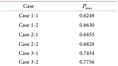
0 =7.Next, we present the computation result. Table 1 shows Pmax for each case. By
check-ing Pmax, we can verify the status of electricity conservation. If Pmax is large, then
there is a trend that consumers conserve electricity. From Table 1, we see the following facts:
1) It is desirable that the initial input (price) is given by u
( )
0 =7.2) Even if one consumer, who is not the leader, conserves electricity, then a contribu-tion to electricity conservacontribu-tion is small.
3) If the leader conserves electricity, then a contribution to electricity conservation is large. Thus, using the PBN-based model, we can analyze real-time pricing systems in a quantitative way.
7. Conclusions
[image:11.595.278.470.599.707.2]In this paper, using a probabilistic Boolean network (PBN), we discussed verification of
Table 1. Computation result.
Case Pmax
Case 1-1 0.6248
Case 1-2 0.6630
Case 2-1 0.6455
Case 2-2 0.6828
Case 3-1 0.7454
1745
real-time pricing systems of electricity. The PBN-based model and PRISM enable us an easy and convenient verification. As one of the verification problems, the reachability problem was considered. In addition, application to model predictive control was also discussed. The proposed method provides us verification/control methods for real-time pricing systems.
There are several open problems. It is significant to develop the identification me-thod of Boolean functions and parameters al( ) ( )i ,bli in (3). Once Boolean functions and parameters can be obtained, the proposed method enables us quantitative analysis. Furthermore, for large-scale systems, there is a possibility that PRISM does not work. In such a case, we may use the assume-guarantee verification technique [17], which is one of the compositional verification techniques. Details are one of the future efforts. It is also significant to consider extending a PBN to a probabilistic system with mul-ti-valued logic functions (see e.g., [18]-[21] for further details about such probabilistic systems). Since the PBN-based model expresses human decision making in the pur-chasing behavior, the proposed method is related to analysis of the consumer behavior in economics. It is important to clarify the relation between the proposed method and the existing method in economics. The proposed method is the first step toward ma-thematical analysis of the consumer behavior.
Acknowledgements
This research was partly supported by JST, CREST and Grant-in-Aid for Scientific Re-search (C) 26420412.
References
[1] Camacho, E.F., Samad, T., Garcia-Sanz, M. and Hiskens, I. (2011) Control for Renewable Energy and Smart Grids. In: Samad, T. and Annaswamy, A.M., Eds., The Impact of Control Technology, IEEE Control Systems Society, New York, USA.
[2] Ruihua, Z., Yumei, D. and Yuhong, L. (2010) New Challenges to Power System Planning and Operation of Smart Grid Development in China. 2010 International Conference on Power System Technology, Hangzhou, China, 24-28 October 2010, 1-8.
[3] Borenstein, S., Jaske, M. and Rosenfeld, A. (2002) Dynamic Pricing, Advanced Metering, and Demand Response in Electricity Markets. Center for the Study of Energy Markets, UC Berkeley.
[4] Roozbehani, M., Dahleh, M. and Mitter, S. (2010) On the Stability of Wholesale Electricity Markets under Real-Time Pricing. Proceedings of the 49th IEEE Conference on Decision and Control, Atlanta, USA, 15-17 December 2010, 1911-1918.
http://dx.doi.org/10.1109/cdc.2010.5718173
[5] Samadi, P., Mohsenian-Rad, A.-H., Schober, R., Wong, V.W.S. and Jatskevich, J. (2010) Optimal Real-Time Pricing Algorithm Based on Utility Maximization for Smart Grid. Pro-ceedings of the 2010 First IEEE International Conference on Smart Grid Communications, Gaithersburg, USA, 4-6 October 2010, 415-420.
http://dx.doi.org/10.1109/SMARTGRID.2010.5622077
Conference of the IEEE Industrial Electronics Society, Vienna, Austria, 10-13 November 2013, 1954-1959.
[7] Tabuada, P. (2009) Verification and Control of Hybrid Systems. Springer, New York, USA.
http://dx.doi.org/10.1007/978-1-4419-0224-5
[8] Adomi, M., Shikauchi, Y. and Ishii, S. (2010) Hidden Markov Model for Human Decision Process in a Partially Observable Environment. Proceedings of the 20th International Con-ference on Artificial Neural Networks, LNCS 6353, Thessaloniki, Greece, 15-18 September 2010, 94-103. http://dx.doi.org/10.1007/978-3-642-15822-3_12
[9] Jong, H.D. (2002) Modeling and Simulation of Genetic Regulatory Systems: A Literature Review. Journal of Computational Biology, 9, 67-103.
http://dx.doi.org/10.1089/10665270252833208
[10] Kauffman, S.A. (1969) Metabolic Stability and Epigenesis in Randomly Constructed Genet-ic Nets. Journal of TheoretGenet-ical Biology, 22, 437-467.
http://dx.doi.org/10.1016/0022-5193(69)90015-0
[11] Shmulevich, I., Dougherty, E.R., Kim, S. and Zhang, W. (2002) Probabilistic Boolean Net-works: A Rule-Based Uncertainty Model for Gene Regulatory Networks. Bioinformatics, 18, 261-274. http://dx.doi.org/10.1093/bioinformatics/18.2.261
[12] Kobayashi, K. and Hiraishi, K. (2014) A Probabilistic Approach to Control of Complex Systems and Its Application to Real-Time Pricing. Mathematical Problems in Engineering, 2014, Article ID: 906717.
[13] Kwiatkowska, M., Norman, G. and Parker, D. (2011) PRISM 4.0: Verification of Probabilis-tic Real-Time Systems. Proceedings of the 23rd International Conference on Computer Aided Verification, LNCS 6806, Snowbird, USA, 14-20 July 2011, 585-591.
[14] Ciesinski, F. and Groesser, M. (2004) On Probabilistic Computation Tree Logic. In: Baier, C., Haverkort, B.R., Hermanns, H., Katoen, J.-P. and Siegle, M., Eds., Validation of Stochas-tic Systems, Springer, Berlin Heidelberg,147-188.
[15] Williams, H.P. (1999) Model Building in Mathematical Programming. 4th Edition, John Wiley & Sons, Ltd., New York, USA.
[16] Kobayashi, K. and Hiraishi, K. (2012) Symbolic Approach to Verification and Control of Deterministic/Probabilistic Boolean Networks. IET Systems Biology, 6, 215-222.
http://dx.doi.org/10.1049/iet-syb.2012.0018
[17] Kwiatkowska, M., Norman, G., Parker, D. and Qu, H. (2010) Assume-Guarantee Verifica-tion for Probabilistic Systems. 16th InternaVerifica-tional Conference on Tools and Algorithms for the Construction and Analysis of Systems, LNCS 6015, Paphos, Cyprus, 20-28 March 2010, 23-37.
[18] Cheng, D. and Xu, X. (2013) Bi-Decomposition of Multi-Valued Logical Functions and Its Applications. Automatica, 49, 1979-1985.
http://dx.doi.org/10.1016/j.automatica.2013.03.013
[19] Kobayashi, K. and Hiraishi, K. (2015) Optimal Control of Probabilistic Logic Networks and Its Application to Real-Time Pricing of Electricity. Mathematical Problems in Engineering, 2015, Article ID: 952310.
[20] Zhao, Y., Li, Z. and Cheng, D. (2011) Optimal Control of Logical Control Networks. IEEE Transactions on Automatic Control, 56, 1766-1776.
http://dx.doi.org/10.1109/TAC.2010.2092290
1747
Appendix A. Probabilistic Computation Tree Logic
In classical propositional logic, truth-value of 0 (false) or 1 (true) is time-invariant. Temporal logic is an extension of propositional logic, and deals with time evolution of truth-value. Since a PBN is a discrete-time system, we also consider temporal logic in discrete-time. First, computation tree logic (CTL) is explained as a class of temporal logics. Next, we introduce probabilistic CTL (PCTL) (see [14] for further details).
In CTL, logical operators and temporal operators are used. The logical operators usually consist of ¬, ∧, ∨, →, and ↔. The temporal operators consists of quan-tifiers over paths A, E and path-specific quanquan-tifiers F, G, X, U. CTL formulas, state formulas, and path formulas are defined as follows:
1) Propositional variables and propositional constants (true or false) are state formu-las.
2) If φ, ψ are state formulas, then ¬φ, φ ψ∧ , φ ψ∨ , φ→ψ , and φ↔ψ are also state formulas.
3) If φ is path formula, then Eφ and Aφ are state formulas.
4) If φ,ψ are state formulas, then Xφ, Fφ, Gφ, and φUψ are path formulas.
5) All state and path formulas consist of the above formulas, and all CTL formulas consist of state formulas.
Next, suppose that φ ψ, are given as propositional variables. Then the meaning of each quantifier over paths is explained as follows:
• Aφ: φ has to hold on all paths starting from the current state (All).
• Eφ: there exists at least one path starting from the current state where φ holds (Ex-ists).
Furthermore, the meaning of each path-specific quantifier is also explained as fol-lows:
• Fφ: φ eventually has to hold (somewhere on the subsequent path) (Finally). • Gφ: φhas to hold on the entire subsequent path (Globally).
• Xφ: φhas to hold at the next state (neXt).
• φUψ: φhas to hold until at some position ψ holds. This implies that ψ will be veri-fied in the future.
In PCTL, the notion of probability is added in CTL, that is, for the CTL formula φ, consider p
( )
φ , ∈ ≤{
, <, , >≥}
, p∈[ ]
0,1 . For example, ≤p( )
φ implies that if φ is true with the probability that is less than or equal to p, then ≤p( )
φ is true, other-wise ≤p( )
φ is false.Finally, the temporal operator F is improved to F≤N. For the propositional variable φ,
Submit or recommend next manuscript to SCIRP and we will provide best service for you:
Accepting pre-submission inquiries through Email, Facebook, LinkedIn, Twitter, etc. A wide selection of journals (inclusive of 9 subjects, more than 200 journals)
Providing 24-hour high-quality service User-friendly online submission system Fair and swift peer-review system
Efficient typesetting and proofreading procedure
Display of the result of downloads and visits, as well as the number of cited articles Maximum dissemination of your research work