Public housing units vs housing vouchers: accessibility, local public goods, and welfare

Munich Personal RePEc Archive

Public housing units vs. housing

vouchers: accessibility, local public

goods, and welfare

Leung, Charles Ka Yui and Sarpca, Sinan and Yilmaz, Kuzey

City University of Hong Kong, Koc University, University of

Rochester

2012

Public Housing Units vs. Housing Vouchers:

Accessibility, Local Public Goods, and Welfare

Charles Ka Yui Leung City University of Hong Kong

Sinan Sarp¸ca Ko¸c University

Kuzey Yilmaz University of Rochester

August 15, 2012

Abstract

We develop a general equilibrium model of residential choice and study the effects of two housing aid policies, public housing units and housing vouchers. Land is differentiated by both residential accessibility and local public goods, and the provision levels of local public goods are determined by property tax revenues and neighborhood compositions. Households differ in their incomes and preferences for local public goods. Housing aid policies are financed by general income taxes. We discuss how the location of public housing units is a fundamental policy variable, in addition to the numbers and sizes of units, and argue that vouchers not only cause less distortion for social welfare compared to public housing, but may also improve overall welfare.

Keywords: Public housing, housing vouchers, housing policy, welfare, residential location choice, local public goods, endogenous sorting.

JEL Classification:H40, D60, H82, R13.

∗_{We thank Henry Pollakowski, three anonymous referees, Eric Hanushek, Ed Olsen, Richard Arnott, John Quigley,}

and Steve Malpezzi, in addition to seminar participants at Bilkent University, the “Macroeconomics, Real Estate Markets, and Public Policy” workshop at Ko¸c University, the Bosphorus Workshop on Economic Design, National Taiwan University Macro Workshop, PGPPE Closing Conference at Bogazici University, and the Econometric Society World Congress in Shanghai for comments and suggestions. Leung thanks the City University of Hong Kong for financial support. Sarp¸ca and Yilmaz acknowledge financial support from The Scientific and Technological Research Council of Turkey. The work described in this paper was partially supported by a grant from the Research Grants Council of the Hong Kong Special Administrative Region, China [Project No. CityU 144709]. We regret that we missed our chance to show the revised version of this paper to John Quigley, who gave us helpful comments and encouragement at the Ko¸c Workshop. His insights, humor, and kindness will always be missed. The usual disclaimer applies. Corresponding Author: Leung, E-mail: kycleung@cityu.edu.hk; Phone: +852 27889604; Address: P7406, Academic Building, City University of Hong Kong, 83 Tat Chee Avenue, Kowloon Tong, Hong Kong.

*Manuscript

1

Introduction

Governments intervene in housing markets all around the world. The forms of these interventions

differ significantly across and within economies.1 _{Although housing aid policies are among the most}

expensive welfare programs in many countries, our understanding of their effects is very limited. The

existing research is mainly empirical and typically evaluates the effects of particular programs on

certain outcomes (e.g., labor supply). Overlooked general equilibrium effects—which may introduce

distortions that counterweigh the benefits measured in partial equilibrium analyses—and

program-specific details can burden such analyses at times. Given the enormous costs of “experiments”

that will provide clear answers to numerous important questions, there are many potential benefits

to studying rich theoretical models that enable thorough comparisons of the effects of alternative

policy proposals.

We develop a general equilibrium model of residential choice and study the effects of two housing

aid policies, subsidized units and housing vouchers. A novel feature of our model is that the land

is differentiated by both residential accessibility and local public goods.2 Households differ in their

incomes and preferences for one local public good, viz. education. The quality of education in a

1

See Smeeding et al. (1993) for cross country comparisons. Whereas the United States tends to provide cash subsidies (Olsen, 2003, comments on the large number of different programs in the U.S.), European countries are more inclined to directly provide physical structures, even when the spending is comparable (Priemus, 2000). In 2001, the United States spent slightly above 1.5% of its GDP on public aid on housing, and the counterpart in France is similar, comprising slightly above 1.7% of the GDP (Laferr`ere and Le Blanc, 2006). Yet the construction-subsidized rental sector (mainly the habitation `a loyer mod´er´e, or HLM in short) accommodates 17% of the households in France, with less than 2% for the U.S. counterpart. Even a simple policy like a cash subsidy can lead to very different outcomes when institutional details differ. For instance, Priemus (2001) states that whereas in the U.S., 100% of the additional rent is paid by tenants, tenants in the Netherlands only pay 25%, and the government is responsible for the rest. Moreover, in the Netherlands, there is no waiting list, and the rent subsidy is perceived as a “right.” As a result, the number of applicants rose from 348,000 in 1976 to 922,000 in 1996. In 1998, there were more than a million households receiving a housing allowance, out of more than 6 million households in the Netherlands. See Malpezzi (2012) for a post-2007-8 evaluation of U.S. housing policies.

2_{Two attributes that households consider when making residential choices, accessibility and local public goods}

neighborhood depends on both the composition of the population in the neighborhood and on the

local educational expenditures. The expenditures are determined by property taxes, the rates of

which are chosen by neighborhood residents through majority voting. The housing aid policies are

financed by general income taxes. We study equilibrium outcomes such as rents, distribution of

households within and across neighborhoods, and school qualities, and pay particular attention to

welfare.

We first present the baseline equilibrium with no government intervention in the housing market.

We observe a sorting of households according to their incomes and preferences in each neighborhood

with respect to location. We also observe a (partial) sorting across neighborhoods. We then

introduce public housing into the model. Public housing programs exhibit large variations from

one market to another, and sometimes even within the same market. We combine some common

elements of the widespread applications to construct the program that we adopt. Public housing

units typically cause property-tax losses to the hosting neighborhood, and households respond by

a stronger sorting across neighborhoods. In addition, the forced location and land consumption

of public housing residents deviate their numeraire consumption and labor supply choices away

from the efficient market allocation. Rents increase in general, and so does the education quality

gap between neighborhoods. The result is a decrease in overall welfare. We then provide public

housing units at alternative locations and find that, in fact, location matters. Our results suggest

that household sorting further increases as public housing units move further from the city center

because the fiscal burden problem created by public housing becomes more serious (and overall

welfare decreases further) as the spatial distribution and choices of households further deviate from

that of the “no-intervention” equilibrium.

As an alternative housing aid policy, we consider providing housing vouchers to the same

partici-pants and present comparisons. We find housing vouchers to be superior to public housing units

in terms of welfare. The difference results mainly from two issues associated with public housing

units: 1. the implications of stronger sorting between neighborhoods as a result of the fiscal burden

problem that arises in the neighborhood that hosts the (property-tax exempt) public housing units;

and 2. the deviations from the efficiency of market allocation caused by forced location and lot size

choices under public housing.

dis-cussions for “in-cash versus in-kind” applies to a more general environment, one that includes

endogenous local public goods, peer group externalities, and accessibility. The framework

devel-oped in this paper can be adapted to compare public housing and/or vouchers to other housing aid

programs, or to compare the outcomes of any single program under different institutional details.

2

The Model

We incorporate a Tiebout economy into Alonso’s (1964) basic land use framework. Households

in a monocentric city work at the Central Business District (CBD hereafter) and reside in the

surrounding area. The distance of home to the workplace matters because of the pecuniary and

time costs of commuting to work. A straight line that goes through the CBD (e.g., a river)

divides the city into two jurisdictions, which we call east (e) and west (w). Each jurisdiction provides its residents a local public good, education. The provision level (quality) of education

in a neighborhood is endogenous, and depends on both the composition of the households in the

neighborhood and local spending (property tax revenues, the rates of which are determined by

majority voting). Agents can move, and hence the tax rates and expenditure levels may differ

between jurisdictions. We discuss this model in further detail below.

2.1 Households

Households choose a neighborhood (east or west), a location in that neighborhood (r, distance to the CBD), lot sizes >0, leisurel∈[0,24], and the consumption level of a composite consumer good

z. The preferences of a household can be represented by the utility functionU(q, s, z, l) =qαsηzγlδ, with q > 0 denoting neighborhood quality. We assume each household has one school-age child and measure neighborhood quality by the quality of education in the neighborhood school. One

member of every household works for an (exogeneous) hourly wageW. Households differ in their wages and in their preferences for school quality. We name the higher income typesskilled workers

(S, earningWS) and the lower income types unskilled workers (U, earningWU < WS), and assume

that skilled workers value education more than unskilled workers do (αS > αU).3

3_{Tastes for education and incomes have been documented as strongly correlated. See Hastings et al. (2008) and}

The city has a dense radial transportation system, and household commuting costs increase with

distance to the CBD: if a household lives r miles away from the CBD, the cost of daily roundtrip commuting is ar dollars (pecuniary cost, a > 0) and br hours (time cost, b > 0), which converts to bW r dollars given the opportunity cost of time.4 We normalize the price of the composite consumption good to one and denote the unit rent of land r miles away from the CBD by R(r). Households pay a property tax on the value of land. Let τ denote the property tax rate as a proportion of daily rent.5 The budget constraint of a household can be written as

z+ (1 +τ)R(r)s+W l=Y(r)≡24W −(a+bW)r. (1)

Given the market rent curves {Re(r), Rw(r)} and quality-tax packages {(qe, τe),(qw, τw)} for each

jurisdiction, typei∈ {S, U} household solves the problem:

max

s,z,l,j∈{e,w} U(q, s, z, l) =q

αi

j sηzγlδ (2)

s.t. z+ (1 +τj)Rj(r)s+Wil=Yi(r).

2.2 Market Rent Curves and Allocation of Land

Land is owned by absentee landlords and auctioned off to the highest bidders. The reservation price

of any given landlord, Ra, is determined by an alternative use of land such as agriculture and is

independent of the location. For a given utility level ¯u, we can find the maximum rent a household is willing to pay per unit of land and optimal lot size r miles away from the CBD by solving the problem Ψ(r,u, q, τ¯ ) = max

s,z,l

n

(Y(r)−z−W l)/((1 +τ)s)

U(q, s, z, l) = ¯u o

to obtain the bid rent

function

Ψi(r,u, q¯ j, τj) =

k1/η

(1 +τj)Wiδ/η

qαi/η_j Yi(r)(η+γ+δ)/ηu¯−1/η (3)

and thebid-max lot size function

s(r,u, q¯ j, τj) = η

(η+γ+δ)(1 +τj)

Yi(r)

Ψi(r,u, q¯ j, τj)

(4)

4_{We ignore non-commute transportation costs and travel costs within the CBD.} 5

where k = _(η+γηη₊γ_δγ₎ηδ+δγ+δ, i ∈ {S, U}, and j ∈ {e, w}.6 At an auction for a particular location r∗,

the winner is the type with the highest bid rent curve at that location. Given the two types in the

model, in each jurisdiction there are two bid rent curves. Theequilibrium rent curve Rj(r) is the

upper envelope of the bid rent curves of two types and the agricultural rent Ra. In equilibrium,

there will be a distance in each jurisdiction r∗

f j, thefringe distance, beyond which no households

reside. Because all bid rent curves are convex and decreasing, the equilibrium rent curve Rj(r)

is also decreasing up to r∗

jf and is constant from that point on. Households with steeper bid

rent curves locate closer to the CBD. Higher income increases the demand for land consumption

and attracts households further away from the CBD, but it also increases the opportunity cost of

commuting time.

Our city is a closed city, that is, population is given exogenously. Let L(r) represent the land density r miles away from the CBD and nj(r) the equilibrium density function of the household

population in jurisdiction j ∈ {e, w}. Suppose that the residents of the land at distance r in jurisdictionj are type i households in equilibrium. If the equilibrium level of utility of the type i

agent,i∈ {S, U}, isu∗

i, thennj(r) = _s(L_r,u(r∗)

i,.). Let ¯NS, ¯NU denote the populations of the respective

types. Thepopulation constraint for typei∈ {S, U}can then be stated as

Z ∞

0

L(r)

sw(r)

I[t∗_w(r) =i]dr+

Z ∞

0

L(r)

se(r)

I[t∗_e(r) =i]dr= ¯Ni, (5)

where t∗_j(r) is a function showing the type of the occupant at distance r in jurisdiction j, and

I[.] is an indicator function that takes the value 1 when the condition in brackets is satisfied and 0 otherwise. The population constraint implicitly assumes that the land market clears in each

jurisdiction (∀r ≤r∗

f j, sj(r)nj(r) =L(r)).

2.3 Neighborhoods

The two neighborhoods may differ in thequality of education andproperty tax rate (qj, τj) packages

they provide. Neighborhood schools are open to the residents of the community only. Admission is

free. Schools are financed by property taxes on residential land. The quality of education q(Π, E) in a neighborhood is determined by (per-student) instructional expenditures E and peer quality

6

Π. For a given group of students, an increase in instructional expenditures increases the quality of

education (∂q/∂E ≥0). Given the equilibrium rent functionRj(r) and equilibrium tax rateτj, we

can calculate the tax base and total tax revenues to find the per-student expenditure in the public

school systemj∈ {e, w}:

Ej =

1

Nj

τj

Z r∗

f j

0

Rj(r)L(r)dr, (6)

whereNj denotes the number of students in neighborhood j.

Different groups of students may benefit differently from a given amount of instructional

expen-ditures. This is captured by the peer quality component Π in our model (∂q/∂Π ≥ 0). Having high-achieving peers may matter in different ways: the students may learn directly from their

peers, they may be motivated by the competition, or the teacher may teach at a higher level or

at a more demanding pace. Because a student’s characteristics are correlated with those of her

parents, achievement at school would be correlated with the background variables of peers.7 We

assume that Π increases with the proportion of skilled households in the neighborhood and use the

following tractable formulation:8

Π =c0+c1 exp

−c2

NU

NS

, c0, c1, c2 ≥0. (7)

We adopt the specification qj =q(Πj, Ej) = ΠjEj for the school quality.

The timing of events is as follows: at the beginning of each period, households make residential

choice decisions, expecting the previous period’s quality-tax rate packages to prevail. They move

in and vote for the tax rate. For a typei household, the most preferred tax rate τ_i∗ = _η−αi_αi is the solution to the indirect utility maximization problem9

τ_i∗ = argmax

τ

V(.) = k

(1 +τj)ηR(r)ηW_iδ

q_jαiYi(r)η+γ+δ (8)

for qj = ΠjEj and Ej = τjR¯j. The households are myopic when voting; they do not consider

the implications of their votes on migration patterns and the composition of neighborhoods. The

7

See Sacerdote (2011) for a long list of studies that document significant effects of peer background on a student’s own test scores in elementary and secondary schools.

8

Alternative specifications give similar results. See, for example, Hanushek and Yilmaz (2007, 2012) and Hanushek, Sarp¸ca, and Yilmaz (2011).

9_{The indirect utility function}

quality tax rate package may be different from what they expected; however, they are stuck until

the beginning of the next period. Then they update their expectations, and the events start over

again. We study the stationary equilibrium, which is attained when no one has an incentive to

relocate in response to the voting results.

Definition: an equilibriumis a set of utility levels {u∗_S, u∗_U}, market rent curves{Re(r), Rw(r)},

quality of education and property tax rate pairs {(qe, τe),(qw, τw)}, household population

distribu-tion funcdistribu-tions {ne(r), nw(r)}, and location-type functions {t∗e(r), t∗w(r)} that show the equilibrium

occupant of the location at distancer in community j such that:

• households’ choices are determined by solving (2);

•the market rent functionRj(r)in each jurisdiction is determined through a bidding process among

different types of households;

• same types of households obtain the same level of utility regardless of their choices;

• the tax rates in each jurisdiction are determined by majority voting by myopic voters;

• local governments’ budgets balance in each jurisdiction,(6);

• labor and land markets clear;

• and the population constraints (5) hold.

2.4 Calibration

The equilibrium of our model can only be calculated numerically.10 We specify parameter values

to match certain statistics from mid-size U.S. cities in 2005. Normalizing the sumη+γ+δ to 1, the solution to the household problem gives the optimal budget shares for leisure, consumption,

and lot size as δ, γ, and η, respectively. In the U.S., the average number of hours of work per week in full-time jobs is 40, and the average annual earnings of workers are $30,104 for high school

graduates and $58,114 for college graduates.11 Accordingly, we set the hourly wages for unskilled

and skilled households asWU = 14 and WS = 27. In a 168 (= 24∗7) hour week, 40 hours of work

implies a 0.762 budget share for leisure, so the budget share of non-leisure (actual expenditures) is (1-0.762).12 _{The data on household expenditures suggest that expenditures on shelter constitute}

10_{The algorithm that is used for solving the models in this paper is available in the web appendix.} 11

U.S. Statistical Abstract.

12

about 20% of the budget of an average household.13 _{This implies budget shares of 4.76%} (=(1-0.762)*20%) for housing and 19% for consumption. We chose the most desired property tax rates

for the two household types as 1.97% (for high valuation) and 1.04% (for low valuation)—slightly higher/lower than the U.S. average of 1.40%—and calibrate the α’s accordingly.14 The average population density in a city with a population of 1 to 2.5 million is about 4.53 people per acre.15

This defines an endogenous calibration target that is achieved by setting agricultural rentRa= $731

per acre per month. The utility function parameters consistent with all of these are αL = 0.014,

αH = 0.021,δ = 0.762, andγ = 0.19.16

(Table 1 about here)

We calculate the commuting costs assuming that households drive to work. The pecuniary cost can

be calculated based on the cost of owning and operating an automobile. In 2004, the pecuniary

cost per mile was $0.56, and we set a= 1.1. Assuming the commuting speed in the city is 20 miles per hour, we setb= 0.13. We assume 1.5 million households populate the city. When computing the equilibrium, we target for a (endogenous) fringe distance (city radius) approximately 15 miles

in each jurisdiction. The proportion of college graduates in the U.S. is about 30%. We expect this

proportion to be slightly higher in a city. Hence, we set the proportion of skilled households to 40%.

We choose the parameters of the school quality function toc0 = 0.1, c1 = 1.3677 andc2 = 0.05743 to match certain endogenous calibration targets to their estimates in the empirical literature.

13

Using data from U.S. Statistical Abstract, the share of shelter in total expenditures can be calculated as 21% for households with incomes less than $70K, 19.6% for those with incomes between $70K–80K, 19% for those with incomes between $80K–100K, and 19.5% for those with incomes $100K and over. With just two income levels in the model, the calibration of budget shares is consistent with these figures.

14

We conducted an additional analysis to check the robustness of our results to changes in the levels ofαi’s and τ∗

i’s. The levels we select forαi’s affect the most desired tax rates of skilled and unskilled households by about±20% or more. This analysis shows that our welfare comparisons are robust to such changes in property tax rates and utility parameters. We report the results from this additional analysis in the web appendix.

15_{U.S. Census Bureau, Population Estimates Files.} 16

2.5 Baseline Equilibrium

Figure 1 displays a map of the city and Table 2 summarizes some properties of equilibrium. Several

observations are immediate: (1) neighborhoods are heterogeneous, both household types exist in

each neighborhood; (2) there is (partial) Tiebout sorting across neighborhoods;17 and (3) there is

income-sorting with respect to distance within neighborhoods: Unskilled households choose smaller

lots closer to the CBD, whereas skilled households live on larger lots away from the CBD.

(Figure 1, Table 2 about here)

The results are intuitive. Costly commuting causes the market rents in each jurisdiction to decrease

in distance to the CBD. Higher income increases the land demand and attracts households further

away from the CBD, where the land is cheaper. High income also increases the opportunity cost of

commuting time, but our calibration suggests that this effect is dominated by the former, consistent

with residential patterns in the U.S. As a result, in each community unskilled households occupy

a semicircle around the CBD. The skilled households reside in a semi-ring that surrounds the

semicircle of unskilled households. The outer end of the skilled households’ semi-ring is the fringe

distance, the land beyond which is left for agricultural use.18 _{The intuition behind heterogenous}

communities is also straightforward: households choose the lot size, distance to the CBD, and the

community (with a given quality of education and a property tax rate) simultaneously. Hence,

lower taxes or lower rents in a community (hence larger lots) can compensate for lower quality of

education and vice versa.

Notice that about 70% of skilled households live in the same neighborhood, constituting a 55%

majority of the population there. As a result, the voting outcome is the higher tax rate. Without

loss of generality, we refer to the higher tax neighborhood as thewest school district throughout

the paper. Because the two neighborhoods have comparable populations, higher taxes and rents

mean higher educational expenditures per student in the west ($3,653 vs $2,027). Also, the peer

17_{The first two observations highlight an advantage of our approach over Tiebout frameworks that do not consider}

accessibility: the partial sorting across heterogeneous communities is consistent with empirical findings on household sorting (e.g., Davidoff, 2005).

18

quality is higher in the west neighborhood; thus the quality of education exceeds that in the east.19

This difference in the quality of education is capitalized into rents; rents in the west are about 25%

higher on average than those in the east.

3

Public Housing

We study two housing aid policies in this and the following sections: government-provided

sub-sidized units and housing vouchers. These programs are financed by uniform income taxes on

earnings ofall households regardless of their location (and participant contributions in the case of

public housing units). Only unskilled households are eligible. The government sets the maximum

number of participantsNP exogenously. If the number of program applicants exceedsNP,

partici-pants are selected by a lottery.20 Table 3 summarizes the main differences between the two policies

we consider.

(Table 3 about here)

3.1 Public Housing Model

The government announces that public housing units will be located betweenrP andrP+wP miles

from the CBD in one of the neighborhoods.21 All unskilled households that consider this to be in

their interest apply, and a lottery selects NP participants in the case of excess demand. The rents

19

The higher tax/expenditure community providing a higher quality of education with higher per-student-expenditure may mislead one to overemphasize the role of per-student-expenditures on school quality. Hanushek, Sarp¸ca, and Yilmaz (2011) show that the existence of a private sector for education breaks the link between expenditures and school quality.

20

Rationing is an important feature of housing aid policies in the U.S. Downs (1991) states“Congress has never provided enough funds for vouchers to make them entitlements, so they must be rationed to a fraction of all eligible households.”Using a panel data set collected by the Housing Authority of the City of Pittsburgh, Epple et al. (2009) estimate that for each family that leaves public housing there are about four families that would like to move into the vacated unit.

21

are determined by the same auction process as described above, with bidders excluding the NP

program participants and including the government. For any location in the public housing band,

the government pays the maximum rent that households would have been willing to pay, had this

land been available to them. This land is then divided into lots with equal sizesP and allocated to

NP participants with subsidized rents. A program participant household pays a fixed priceRP as

its program contribution. Denote the income tax rate by θ. This policy reduces a public housing resident’s problem to leisure-consumption choice only:

max

z,l UP(qe, sP, z, l) =q αU e s

η

Pzγlδ s.t. (9)

z+RP + (1−θ)WUl=YP(r) = 24(1−θ)WU−(a+b(1−θ)WU)r,

whereas other households of typei∈ {S, U}solve the original problem (2) in the presence of income taxes:

max

s,z,l,j∈{e,w} U(q, s, z, l) =q

αi

j sηzγlδ s.t. (10)

z+ (1 +τj)Rj(r)s+ (1−θ)Wil=Yi(r) = 24(1−θ)Wi−(a+b(1−θ)Wi)r,

taking rents and neighborhood quality-tax pairs as given.22

The cost of public housing is financed by income tax revenues and participant contributions, and

equals the sum of rents and any payments to the local government. Public housing units are

exempt from property taxes; a payment—known asPayment in Lieu of Tax, or PILOT—is made

to compensate the local government in the east for some of the property tax revenue that it loses,

in recognition of the services it provides to public housing residents.23 _{The time constraint of}

a household gives the labor supply as all of the time except leisure and commute time: n = 24−l−br. The solution to (10) gives the optimal leisure of a household residing at distance r as

22

An incentive problem arises when public housing residents do not pay property taxes, as their most preferred tax rate would be 100% when voting. Even though the equilibrium described in the next section is not affected by this, there may be some alternative specifications that may result in different types of equilibria depending on whether public housing residents are allowed to vote or not. For consistency, we assume that public housing residents vote for the same tax rate as other unskilled households.

23_{Given that public housing complexes are built/subsidized with public money (and that their rent incomes are}

l_i∗(r) = δ₍₁₋Yi_θ(r_)Wi) for i ∈ {S, U}. For a household that lives in public housing, optimal leisure is

l_P∗(r) = _δ+δ_γYP₍₁₋(r_θ)−_)WURP. We can define at∗_j(r) function that shows the type of occupant at distancer

in jurisdictionj (whether skilled, unskilled, or in public housing). Let I[.] be an indicator function that takes the value 1 when the condition in brackets is satisfied and 0 otherwise. The public

housing program budget constraint is:

Z rP+wP

rP

Re(r)L(r)dr+P ILOT =θ

X

j∈{e,w}

" Z r∗_{f j}

0

L(r)

sj(r)

X

i∈{S,U,P}

I[t∗_j(r) =i](24−l∗_i(r)−br)Wi

! dr

#

+NPRP. (11)

The LHS adds up the total rent cost of the public housing band and the payment to the local

government, the choice of which we discuss below. Consider the first term on the RHS: the inside

summation identifies which household type resides at a particular location and calculates their

labor income in equilibrium. The integral calculates the total labor income using the household

density at that location. The outside summation adds the labor income of two communities. A

fraction θ of this gives us the income tax revenues. The second term on the RHS is the sum of participant contributions. Equilibrium now also requires program budget constraint (11) holds.

3.2 Equilibrium

We first study a model in which the government provides public housing units on the land that

is between 4 and 6 miles away from the CBD in theeast neighborhood. This causes most skilled

households to reside in the west, which then becomes the higher rent/tax/school quality

neighbor-hood.24 In the baseline equilibrium unskilled households lived in this band in the east, and the lot

sizes ranged from 0.109 to 0.154 acres (at 4 and 6 miles away from the CBD) with an average lot

size of 0.128 acres. The average monthly rent was $3,520 per acre. A public housing unit measures

0.160 acres now. This is about 25% larger than the average unit within that band in the baseline

equilibrium. This band accommodates about 15% of all unskilled households. We exogenously

set the income tax rate at 0.57% to match the endogenous calibration target for the participant

contribution for public housing of $339 so that the utility increase from public housing is equivalent

24

to that from a 10% income subsidy in equilibrium and (11) holds.

In practice, the basis for deciding upon an appropriate PILOT amount varies across municipalities.

One of the recommendations in Lunney (2009) is to“lower the property value on which the tax rate

is assessed by basing the assessment on actual income and expenses rather than on potential market

rate figures.”A typical public housing complex would have a lower rent income and higher operating

costs than a comparable private rental complex. Kenyon and Langley (2010) report that “Some

(municipalities) ask tax-exempt institutions to pay a specific proportion of the property taxes the

institution would owe if taxable. (...) in many cases PILOTs are completely ad hoc and negotiated

without any apparent basis.” These and other resources suggest that property taxes collected over

total rent income of the public housing program (P ILOT = τeNPRP) would be an appropriate

choice. With our calibration, this corresponds to 42% of the property taxes that would be owed in

equilibrium if the public housing band was fully taxable (for example, the city of Boston seeks 25%,

Kenyon and Langley, 2010). Bowman, et al. (2009) estimate that the state-level foregone property

tax revenues because of PILOTs range between 1.5% to 10% of property tax revenues, and the

national average is around 5%. Our specification implies a 3.42% loss. Choosing a smaller PILOT

would make public housing residents even less desirable neighbors, strengthening our arguments

against public housing that will follow. (We comment on the implications of choice of a larger

PILOT in the conclusion.)

We present the welfare effects of this policy in the first row of Table 4. Our welfare measure is the

change in rents necessary to provide households with their utility level in baseline equilibrium. A

negative number indicates that the household type is worse off, because rents need to be decreased

to make those households indifferent to the baseline allocation. As a measure of the change in

overall welfare, we calculate the change in rents necessary to keep aggregate utility at the baseline

equilibrium level and present it in column 4 (AU). Public housing residents are better off, whereas

all other households are worse off compared to baseline equilibrium; overall welfare (as measured

by AU) is lower.

(Table 4 about here)

Table 5 presents some properties of the new equilibrium, and Figure 2 displays a map of the city.

the west (up from 69% in baseline) and constitute the majority there.

(Figure 2, Table 5 about here)

Rents are higher than those in the baseline equilibrium in both neighborhoods. The intuition

is straightforward: the public housing policy removes a substantial amount of would-be-inhabited

land from the private market. The non-recipients, who are either the skilled or the less fortunate

unskilled workers, compete for the remaining land. However: 1. the average income of these

households—which affects their willingness to pay for land—that compete in the private market is

higher than before (because the households who left the private market are exclusively unskilled);

and 2. the amount of accessible land is less than before (because public housing took out more

land from the market than its residents would obtain on their own, if they had a choice). As a

result, other things being equal, one would expect to see higher rents in equilibrium. However,

other things are not equal, as there is also a fiscal burden issue: the property tax revenues from

the public housing band are less than what would be collected from the same area without tax

exemptions. This makes public housing residents undesirable neighbors, and the magnitude of this

problem increases in the gap between the property tax revenues at market rents and the PILOT.

For skilled households (with stronger preferences for education), the west is now a better option

than before: the marginal effects of a tax dollar on per-student expenditures are higher. As a result,

sorting is stronger, and the difference in quality of education is higher between two neighborhoods

compared with the baseline equilibrium, as both the spending and the peer quality in the west

(east) are higher (lower) than before. The computed equilibrium quantifies the described effects.

We also observe that the public housing residents decrease their labor supply by about 6.5% on

average to 38.6 hours per week, down from 41.3 hours in baseline equilibrium. This is a result of

two effects: 1. income taxes decrease the relative price of leisure; and 2. rent subsidy expands the

budget set for leisure and consumption, but not for housing, resulting in a disproportionate increase

in the consumption of the first two. Additional analysis confirms the presence of such a strong effect

under several alternative formulations.25 These findings are consistent with the empirical findings

on housing aid policies and labor supply.26

25_{Results from the additional analysis are available in the web appendix.} 26

The Size of a Public Housing Unit

In the analysis presented above, a public housing unit is 25% larger compared with the average

unit that was on the band now occupied by public housing units in the baseline equilibrium. Our

results regarding welfare, however, are not driven by this particular choice of size. Note that if

they were given a choice, public housing residents would now choose a lot that is slightly larger

than their choices in the baseline equilibrium because of the income effect of the subsidy. A further

increase in the size of public housing units, however, may hurt the public housing residents, as the

net cost (subsidized rent) has to increase with the size for the program budget to hold: first, the

lots are larger, and second, the overall level of rents is higher because the removal of accessible

land from the private market is more excessive than before. Note that although the population

density decreases in the east with larger public housing units, the property tax loss becomes a larger

concern, as it applies to a larger area in the neighborhood. (We would see the opposite effects with

smaller units.)

Within-district Location of Public Housing Units

In the analysis presented above, the public housing units are provided 4 miles away from the CBD.

At that location, a public housing unit is 25% larger than a typical lot at the same location in the

baseline model (and is close in size to what the public housing residents would obtain on their own

with the income effect of the subsidy). We utilize the spatial features of our model by comparing the

welfare outcomes with public housing units provided at different locations. To isolate the effects of

location, we now keep the sizes and the number of subsidized units—hence the total area occupied

by public housing—the same while varying the distance of the public housing band to the CBD.

If moved closer to the CBD, the (same-size) public housing unit becomes larger compared with a

typical lot around that location. Although the commuting costs decrease for the public housing

residents, their rents are higher closer to the CBD, and the subsidy covers a smaller share of this

higher rent. Public housing also replaces a larger number of households that would occupy the

same area without public housing. This has two implications: first, property-tax loss in the east

increases (because the market rents are higher when closer to the CBD, but PILOT is proportional

to subsidized rents); and second, the number of households competing for land in the private market

would observe the opposite effects as the public housing units are moved away from the CBD.)

Welfare Comparisons

How welfare is affected by changes in the size and location of public housing units depends on

the relative magnitudes of the effects described above, the associated implications on the sorting

of households in response, and the resulting levels and differentials of rents, tax rates, and school

qualities in equilibrium.

Rows 2 to 6 of Table 4 summarize the welfare changes associated with the size of a public housing

unit ranging from 25% smaller (–25%) to 75% larger (+75%) compared with the average unit on

the area occupied by public housing band in the baseline equilibrium. The last column shows that

overall welfare decreases as we move away from our initial choice of 25% larger in either direction.

Varying the lot size between –25% and +25% seems to have only a small effect on public housing

residents’ welfare, but increases beyond +25% make the public housing residents significantly worse

off as: 1. they would be forced to obtain lots that are too large compared to their optimal choice

under this income effect; 2. holding total government subsidies and the number of public housing

residents constant, the share of subsidies in this forced lot-size consumption would be too small.

Rows 7 to 10 of Table 4 summarize the welfare effects when public housing units are provided at 0,

2, and 6 miles away from the CBD. We find that the welfare of public housing residents increases

as public housing units are provided further away from the CBD, suggesting that the decrease in

the net cost of the land outweighs the increase in commuting costs.

A deviation from our initial choice of +25% or from our initial choice of four miles in either direction

hurts households outside of public housing, because of the changes in the magnitude of the fiscal

burden problem (arising from changes in the amount of property-tax loss and population density)

and the implied general equilibrium effects described above.

In each of the cases we have studied, the total utility gain of public housing residents is smaller

than the total utility loss of the rest of the population, so the change in overall welfare (as measured

4

Housing Vouchers

4.1 Voucher Model

Instead of providing physical units with subsidized rents, the government can simply redistribute

the income tax revenues to low-income households in the form of housing vouchers. In this scenario,

each of theNP program participants obtains a voucher towards rent with the amountνP. For the

government budget to balance, income tax revenues must equal the total amount of these vouchers:

NPνP =θ

X

j∈{e,w}

" Z r∗_{f j}

0

L(r)

sj(r)

X

i∈{S,U,P}

I[t∗_j(r) =i](24−l∗_i(r)−br)Wi

! dr

#

(12)

A household’s problem is the same as the one in (10), but a voucher recipient’s housing expenditures

are those exceedingνP only. This is equivalent to creating a third household type with the same

preferences as unskilled households, but with the kinked budget constraint

z+max{0,(1 +τj)Rj(r)s−νP}+WUl=YP(r) = 24(1−θ)WU−(a+b(1−θ)WU)r. (13)

Because household utility increases in lot size, no household will spend less on housing than the

voucher amount. Whether the household will spend more depends on the voucher amount and some

model parameters. The leisure choice of a voucher recipient is l∗_P(r) = δYP₍₁₋(r_θ)+_)WUνP if the household spends greater than the voucher amount, andl∗

P(r) = γ+δδ YP(r)

(1−θ)WU otherwise. The land is allocated

according to the competitive auction mechanism described in Section 2. An additional equilibrium

condition is that the program budget (12) holds.

4.2 Equilibrium

For comparison, we keep the (number of) recipients and the tax rate the same as the public housing

policy; this implies a housing voucher worth $227 per month.27 _{Figure 3 provides a map of the city}

27

and Table 6 summarizes some properties of equilibrium. Vouchers shift land demand, increasing

rents in both neighborhoods. The equilibrium rents, however, are lower than those under public

housing policy, because there is no excessive removal of accessible land from the market as there is

under public housing.

Sorting of households is stronger than that under the baseline equilibrium, close to the public

housing equilibrium levels: 74% of skilled households live in the west (as opposed to 69% in baseline)

and constitute a 56% majority there. The major cause of this is the increase in land demand in the

east: all voucher recipients reside in the east (where unskilled households are a majority) because of

their weaker preferences for education. The quality of education in the west is slightly higher than

both the baseline and public housing models, because of both sorting and the higher expenditures.

A policy maker concerned with education of the poor may prefer vouchers over public housing: the

quality in the east, the poorer neighborhood, is higher than that under the public housing model.

The fiscal burden problem we described in the public housing units section is of no concern here, as

voucher recipients still pay property taxes at the market rent level. However, households without

vouchers are hurt by both the higher rents and income taxes. The equilibrium utility levels of

non-recipients (both skilled and unskilled households) are higher than those under public housing,

but lower than baseline equilibrium levels. The (average) utility level of voucher recipients falls

below that of public housing recipients. We present the change in household welfare according to

their types in the last row of Table 4. The welfare loss to non-recipients is less than that under

public housing policy, and the change in total welfare (as measured by AU) is positive.

(Figure 3, Table 6 about here)

Income taxes hurt work incentives by decreasing the relative price of leisure. The income effect of

vouchers also allows recipients to increase their leisure consumption. But voucher recipients work

more than public housing recipients (42 vs. 38.6 hours/week). This should not be puzzling: the

public housing program also creates an income effect, but by restricting households’ location-lot size

choices and their housing expenditures, it also causes a disproportionate increase in consumption

of the other two commodities available for purchase, the composite good and leisure. Housing

voucher recipients are not restricted in terms of their residential choices, they reside further away

though they work less than the typical unskilled resident living at the same distance in baseline

equilibrium—a result of the income effect caused by the voucher—they work longer hours than

they would if they received public housing instead.

4.3 A Note on Desegregation

We have discussed several reasons a housing voucher program might be preferred over a public

housing program with the same budget. Another advantage of housing vouchers over public housing

units is that the vouchers do not impose restrictions on households’ location choices. Hence, a policy

maker with concern over the patterns of household sorting across neighborhoods may be particularly

interested in how housing vouchers can influence these patterns.

The equilibrium neighborhood compositions under the two programs are, however, almost identical

in the above analysis. The west community provides a higher quality of education at the cost of

higher taxes on land consumption. The skilled households have stronger preferences (and willingness

to pay) for education compared with voucher recipients, so they outbid the voucher recipients on the

west land away from the CBD. However, unskilled households without vouchers value proximity to

the CBD and outbid voucher recipients on the west land close to the CBD. The unskilled households

demand smaller lots than voucher recipients and therefore are not as affected by larger taxes as

much as voucher recipients who demand relatively larger lots. As a result, voucher recipients are

not observed residing in the west. We have also mentioned that increasing the number of voucher

recipients without changing the income tax rates resulted in a similar equilibrium.

We conducted an additional analysis with alternative parameterizations that may allow us to

ob-serve voucher recipients in the west. Increasing tax rates while keeping the number of recipients

the same did not cause enough increase in the bids of voucher recipients in the west. We have

observed, however, that it is possible to induce voucher recipients residing in the west with both

a larger program size and a larger income tax rate, increasing the voucher recipients’ land bids in

both neighborhoods and allowing them to outbid some households in the west. We present the

spatial distribution of households in the equilibrium of one such model in Figure 4, in which 25% of

unskilled households receive housing vouchers for $537 per month. This program is financed by an

income tax rate of 1.5%. In the equilibrium of this model, about one fifth of the voucher recipients

the CBD and the skilled households’ semi-ring. Other aspects of the equilibria remain qualitatively

the same for our purposes, so we refrain from a detailed discussion here.28

(Figure 4 about here)

5

Concluding Remarks

Green and Malpezzi (2003) survey a vast literature on the housing market and housing policies in the

U.S., and argue that“Most economists like vouchers because they are generally more efficient than

other programs. (...) But in the United States, political support is generally stronger for programs

tied more closely to the consumption of specific goods (housing, food, and medical care) than for

income support.” This paper attempts to contribute to this related debate. In particular, this

paper explicitly highlights the importance of the location of public housing to equilibrium outcomes

such as rents, neighborhood compositions, educational opportunities, labor supply decisions, and

social welfare. We explain the channels through which such location effects work. Using a rich

general equilibrium model that combines land use theory with a Tiebout framework, we provide

a comparison of public housing and housing voucher policies, and conclude that vouchers not

only cause less distortion for social welfare compared with public housing, but they also improve

overall welfare. The difference between the two policies is mainly driven by the implications of: 1.

property-tax losses of the neighborhood under public housing; and 2. the forced location and lot

size choices under public housing. Therefore, even if the fiscal burden problem of public housing is

solved (e.g., with higher PILOTs), vouchers may still be preferred because of the freedom of choice

in location and lot sizes. The results of our analysis are consistent with the findings from previous

studies that compare in-kind versus in-cash welfare programs, verifying their validity in a richer

framework with accessibility, local public goods, and peer group externalities.

We also find that public housing policies tends to discourage the labor supply, especially for the

unskilled workers who reside in public housing, as some empirical literature has suggested. Voucher

recipients work the same hours as they did before the vouchers. This seems to strengthen the

in-cash rather than in-kind arguments even further. Additional analysis (the results of which are

available in the web appendix) reveals that our findings are robust to changes in the levels for utility

28

parameters (which determine most desired property tax rates) as well as to the incorporation of a

housing industry.29

In many countries, central governments contribute to the financing of local public goods and services

in differing extents. If the share of local financing decreases in our model, the sorting would be

weaker, as it becomes less effective on the local provision level. An implication is that unskilled

households constitute the majority in both neighborhoods above a certain share of central financing.

In that case, the voting outcome would be the lower tax rate in both neighborhoods, and the quality

difference between the neighborhoods would be less. Another implication is that desegregation could

be obtained more easily with vouchers than as presented in this paper. Future work will investigate

these issues in detail.

References

Alonso, W. (1964). Location and Land Use. Cambridge, MA: Harvard University Press.

Bingley, P., Walker, I. (2001). Housing subsidies and work incentives in Great Britain. Economic Journal, 111(471), 86-103.

Bowman, W., Cordes, J., Metcalf, L. (2009). Preferential tax treatment of property used for social purposes: Fiscal impacts and public policy implications. In Erosion of the property tax base: Trends, causes, and consequences, ed. Augustine, N. Bell, M., Brunori, D., and Youngman, J. 269294. Cambridge, MA: Lincoln Institute of Land Policy.

Davidoff, T. (2005). Income Sorting: Measurement and Income Decomposition. Journal of Urban Economics

58, no.2 (September):289-303.

de Bartolome, C., Ross., S. (2003). Equilibria with local governments and commuting: Income sorting vs income mixing. Journal of Urban Economics 54:1-20.

Downs, A. (1991). Deciding How to Use Scarce Federal Housing Aid Funds,Housing Policy Debate, (2) 2, 439-463.

Ellickson, B. (1971). Jurisdictional Fragmentation and Residential Choice. American Economic Review 61, 334-339.

29

Epple, D., Filimon, R., Romer, T. (1984). Towards an Integrated Treatment of Voting and Residential Choice. Journal of Public Economics 24, 281-308.

Epple, D., Filimon, R., Romer, T. (1993). Existence of Voting and Housing Equilibrium in a System of Communities with Property Taxes. Regional Science and Urban Economics 23:585-610.

Epple, D., Geyer, J., Sieg, H. (2009) Excess Demand and Rationing in Equilibrium in the Market for Public Housing, Working Paper.

Fernandez, R.; Rogerson, R. (1996). Income distribution, communities, and the quality of public education.

Quarterly Journal of Economics 111, no.1: 135-164.

Fujita, M. (1999). Urban Economic Theory: Land Use and City Size. Cambridge Univ. Press, Cambridge, MA.

Glaeser, E., Kahn, M., Rappaport, J. (2000). Why Do The Poor Live in Cities? NBER Working Paper 7636.

Green, R., Malpezzi, S. (2003). A primer on U.S. Housing Markets and Housing Policy. AREUEA monograph series, Washington, D.C.: Urban Institute.

Hanushek, E.; Sarp¸ca, S.; Yilmaz, K. (2011). Private Schools and Residential Choices: Accessibility, Mobility, and Welfare. The B.E. Journal of Economic Analysis & Policy Vol. 11: Iss. 1 (Contributions), Article 44.

Hanushek, E., Yilmaz, K. (2007). The complementarity of Tiebout and Alonso. Journal of Housing Eco-nomics, 16(2), 243-261.

Hanushek, E., Yilmaz, K. (2012). Household location and schools in metropolitan areas with heterogeneous suburbs: Tiebout, Alonso, and government policy. Journal of Public Economic Theory, forthcoming.

Hastings, J.; Kane, T. ; Steiger, D. (2008). Heterogeneous Preferences and the Efficacy of Public School Choice.

Hulse, K., Randolph, B. (2005). Workforce disincentive effects of housing allowances and public housing for low income households in Australia. European Journal of Housing Policy, 5(2), 147-165.

Kenyon, D., Langley, A. (2010). Payments in Lieu of Taxes. Balancing Municipal and Nonprofit Interests. Lincoln Institute of Land Policy. Cambridge, MA.

Laferr`ere, A., Le Blanc, D. (2006). Housing policy: low-income households in France. In: R. Arnott and D. McMillen (Eds.), A Companion to Urban Economics, Oxford: Blackwell Publishing.

Lunney, F. (2009). Payment in Lieu of Taxes Programs (PILOTs) for Affordable Housing Complexes. Alliance for Housing Solutions Report. Accessible at: http://www.allianceforhousingsolutions.org/

Malpezzi, S. (2012). U.S. Rental Housing markets and policies: before and after the Great Financial Crisis, University of Wisconsin, Madison.

Mills, E. S. (1972). Studies in the Structure of the Urban Economy. Baltimore, MD. Johns Hopkins University Press.

Muth, R. F. (1969). Cities and Housing. Chicago: University of Chicago Press.

Journal of Public Economic Theory. 1, no. 1, 5-50.

Nechyba, T. (2000). Mobility, targeting, and private-school vouchers. American Economic Review 90, no.1 (March):130-146.

Olsen, E. (2003). Housing Programs for Low-Income Households. in Means-Tested Transfer Programs in the United States, ed., Robert Moffitt, National Bureau of Economic Research, Chicago: University of Chicago Press.

Olsen, E., Tyler, C., King J., Carrillo, P. (2005). The effects of different types of housing assistance on earnings and employment. Cityscape: A Journal of Policy Development and Research, 8(2), 163-187.

Priemus, H. (2000). Rent subsidies in the USA and housing allowances in the Netherlands: worlds apart.

International Journal of Urban and Regional Research, 24, 700-712.

Priemus, H. (2001). Poverty and housing in the Netherlands: a plea for tenure-neutral public policy. Housing Studies, 16, 277-289.

Sacerdote, B. (2011). Peer Effects in Education: How Might They Work, How Big Are They and How Much Do We Know Thus Far? In: Hanushek, E.; Machin, S.; Woessmann, L.(Eds.),Handbook of the Economics of Education, Volume 3, Elsevier.

Smeeding, T.M., Coder, J., Fritzell, J., Hagenaars, A.M., Hauser, R., Jenkins, S., Saunders, P., Wolfson, M. (1993). Poverty, Inequality, and Family Living Standards Impacts Across Seven Nations: The Effect of Noncash Subsidies for Health, Education, and Housing. Review of Income and Wealth 39(3), 229-256.

Straszheim, M. (1987). The Theory of Urban Residential Location. in Handbook of Regional and Urban Economics, J.V.Hendersson and J.F.Thisse, eds. New York: Elsevier.

Tiebout, C.M. (1956). A pure theory of local expenditures. Journal of Political Economy 64-5, 416-424.

Table 1: Calibration Parameters

δ 0.762

γ 0.19

η 0.048

WU 14

WS 27

αL 0.014

αH 0.021

a 1.1

b 0.13

c0 0.1

c1 1.3677

c2 0.0574

NS/(NS+NU) 0.40

Table 2: Baseline Equilibrium

West East Average Monthly Rent (per Acre) $2729 $2194 Average Rent in S area $2204 $1433 Average Rent in U area $5416 $3368 Average Lot Size S (Acres) 0.791 1.209 Average Lot Size U 0.173 0.275 Property Tax Rate 1.97% 1.04%

School Quality 14 7

Distribution of Households Across Neighborhoods

S 69% 31%

U 42% 58%

Neighborhood Population Breakdown

S 53% 26%

U 47% 74%

Table 3: Housing Aid Policies

Public Housing Units Housing Vouchers Location & Lot size Choice By policy-maker By voucher recipients Rent Paid Fixed, below market rent Reduced by voucher amount Property Taxes Households do not pay property

taxes, the program makes a pay-ment in lieu of taxes (PILOT)to the local government

Table 4: Welfare

S U P AU

Public Housing -5.64 -5.39 85.67 -0.35

-25% -9.24 -5.71 81.16 -2.41 0 -9.28 -6.45 86.63 -2.57 Size of Public Housing +25% -5.64 -5.39 85.67 -0.35 +50% -9.55 -8.04 63.51 -4.49 +75% -9.72 -8.81 44.80 -5.87 0-4.47 miles -9.83 -9.20 33.53 -6.71 2-4.90 miles -9.61 -8.41 52.72 -5.23 Location of Public Housing 4-6.00 miles -5.64 -5.39 85.67 -0.35 6-7.48 miles -9.29 -6.20 88.37 -2.37

Vouchers -3.29 -3.31 59.01 0.54

Table 5: Public Housing Income Tax Rate: 0.57%

West East Average Monthly Rent (per Acre) $2764 $1955 Average Lot Size S (Acres) 0.770 1.261 Average Lot Size U 0.165 0.301

Average Lot Size P - 0.320

Property Tax Rate 1.97% 1.04%

School Quality 14.15 6.02

Distribution of Households Across Neighborhoods

S 75% 25%

U 41% 59%

(14% P)

Neighborhood Population Breakdown

S 55% 22%

U 45% 78%

Table 6: Housing Vouchers Income Tax Rate: 0.57%

West East Average Monthly Rent (per Acre) $2741 $2186 Average Lot Size S (Acres) 0.771 1.246 Average Lot Size U 0.166 0.247

Average Lot Size V - 0.423

Property Tax Rate 1.97% 1.04%

School Quality 14.25 6.56

Distribution of Households Across Neighborhoods

S 74% 26%

U 39% 61%

(14% V)

Neighborhood Population Breakdown

S 56% 22%

U 44% 78%

b

CBD

8.47 mi. U

5.02 mi. S 5.68 mi.

U 8.33 mi.

S

West East

Figure 1: Spatial Distribution of Households in the Baseline Equilibrium. The outer semi-rings (marked by S) are the areas in whichskilled households reside. The inner semicircles (marked by U) are the areas in

b

CBD

8.95 mi. U

4.23 mi. S 5.54 mi.

U 8.71 mi.

S

West East

Figure 2: Spatial Distribution of Households in the Public Housing Equilibrium. The outer semi-rings (marked by S) are the areas in whichskilled households reside. The inner semicircles (marked by U) are the areas in whichunskilled households reside. The shaded semi-ring is the public housing band between 4

b

CBD

7.21 mi. U

1.65

P S

4.43 5.39 mi.

U 8.69 mi.

S

West East

Figure 3: Spatial Distribution of Households in the Vouchers Equilibrium. The outer semi-rings (marked by S) are the areas in whichskilled households reside. The inner semicircles (marked by U) are the areas in

b

CBD

6.08 mi. U

3.03

P S

3.61 6.08 mi.

U 5.92 mi.

S

West East

Appendix to “Public Housing Units vs. Housing Vouchers:

Accessibility, Local Public Goods, and Welfare”

Charles Leung, Sinan Sarp¸ca, Kuzey Yilmaz

29.06.2012

NOT FOR PUBLICATION,

ACCESSIBLE AT:

http://a.permanent.url.will.be.assigned/web_appendix.pdf

A.1 Robustness and Extensions

A.1.1 Utility Parameters and Tax Rates

The most desired property tax rates for the two household types are chosen to be slightly higher/lower than the U.S. average of 1.40%, and the utility parametersαH and αL are calibrated according to

equation (8) in the paper. We conduct an additional analysis with alternative specifications for the levels ofαi’s, which affect desired tax rates by about±20% or more. Table A.1 reports

representa-tive results results from these alternarepresenta-tive specifications along with the original specification given in the middle row of each panel. An inspection of the columns reporting the changes in overall welfare (AU) under two policies shows our findings are robust to such changes in property tax rates.

Table A.1: Welfare II - Property Tax Rates

Public Housing Vouchers

(αH, αL;τH∗, τL∗) S U P AU S U P AU

(.018, .014; 1.52, 1.04) -4.85 -5.18 81.74 -0.34 -2.93 -2.72 59.42 1.03

(.021, .014; 1.97, 1.04) -5.64 -5.39 85.67 -0.35 -3.29 -3.31 59.01 0.54

(.024, .014; 2.54, 1.04) -5.26 -5.20 82.04 -0.25 -3.01 -2.72 59.42 0.97

(.021, .012; 1.97, 0.84) -4.89 -4.90 76.36 -0.17 -2.99 -2.73 59.50 0.99

(.021, .014; 1.97, 1.04) -5.64 -5.39 85.67 -0.35 -3.29 -3.31 59.01 0.54

(.021, .016; 1.97, 1.26) -5.20 -5.49 88.16 -0.08 -3.00 -2.78 59.23 0.96

A.1.2 Labor Supply

One of our findings is that households decrease their labor supply when provided with public housing units. In this section we provide representative results from additional analysis in which we vary: 1. The sizes of public housing units; 2. The location of the public housing units; 3. Utility (and tax rate) parameters. Table A.2 summarizes average working hours per week, comparing the labor supply of public housing residents and housing voucher recipients to labor supply of the households that live on the public housing location in benchmark equilibrium.1 One row in each panel (+25%, 2-4.90, and (.014, .021), in bold) represents the original model for reference. Public housing recipients work less than voucher recipients (The only exception arises when public housing is built at the CBD and a public housing resident’s travel cost becomes zero).

Table A.2: Average Weekly Labor Supply of Housing Aid Participants (hours/week)

Benchmark Public Housing Housing Vouchers

Size

-25% 41.2 35.6 42.0

0 41.2 37.3 42.0

+25% 41.3 38.6 42.0

+50% 41.3 40.6 42.0

+75% 41.3 42.3 42.0

Location

0-4.47 40.7 42.5 42.0

2-4.90 40.9 41.1 42.0

4-6.00 41.3 38.6 42.0

6-7.48 41.7 37.2 42.0

(α_L, α_H)

(.012,.021) 41.3 39.1 41.7

(.014,.018) 41.3 39.0 41.7

(.014,.021) 41.3 38.6 42.0

(.014,.024) 41.3 38.9 41.7

(.016,.021) 41.3 38.8 41.7

A.1.3 Vouchers for All Unskilled Households

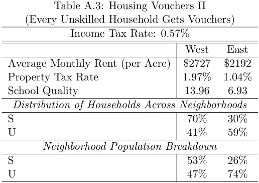
Rationing of housing vouchers to a fraction of eligible households is consistent with the practices in the U.S. (Downs, 1991). The lottery specification in the paper has the additional benefit of keeping the program size the same as under public housing. An alternative implementation is to provide vouchers to every household below a certain income level. With just two income levels in the model, this means providing vouchers to all unskilled households, increasing the number of program participants from 9% to 60% of the population. Holding income tax rate constant decreases the voucher amount to $34 per household. The findings of this exercise given in Table A.3 are quite similar to those of the lottery specification in the paper.

Table A.3: Housing Vouchers II (Every Unskilled Household Gets Vouchers)

Income Tax Rate: 0.57%

West East Average Monthly Rent (per Acre) $2727 $2192 Property Tax Rate 1.97% 1.04%

School Quality 13.96 6.93

Distribution of Households Across Neighborhoods

S 70% 30%

U 41% 59%

Neighborhood Population Breakdown

S 53% 26%

U 47% 74%

A.1.4 Housing Industry

Our framework is based on Alonso’s model (1964) which assumes that each household manages the construction of its house by itself. An alternative approach is Muth’s model (1969) in which households derive utility from consuming housing spaceH, produced by competitive firms using Λ units of land andK units of capital with the production function:

H =AKaΛ1−a ₍₁₎

fora∈₍₀,1) andA >0. Then as land gets more expensive closer to the CBD, the share of capital to land in the construction of housing space increases, i.e., taller/multi-unit buildings are observed.

We incorporate this housing industry to our framework, and repeat the analysis presented so far in this paper. This change in the formulation does not alter our qualitative findings regarding welfare comparisons, while adding considerable complexity to the analysis. We solve the equilibrium without government intervention (benchmark), with public housing, and with housing vouchers. We calibrate the parameters of the housing production function so thatthe ratio of housing space to land is about 16 near the CBD and 1 near fringe in the benchmark model.2

We initially locate the public housing units at 4 miles away from the CBD, keeping the ratio of housing space to land at the benchmark level at this distance (about 4). We set the public housing unit size same as the average unit in the same area in benchmark. We have also solved alternative models with: 1. The public housing unit size 25% smaller and 25% larger than the average unit in the same area in benchmark; 2. The ratio of housing space to land is 3 and 5; 3. The location of public housing units at 3 and 5 miles away from the CBD. We summarize results from this analysis in Table 7 below. The middle rows in top three panels (titled as “same,” “4,” “4 miles”) represent the main public housing model, and the very bottom row in the table presents the welfare implications of the voucher model with housing industry.

An inspection of Table A.4 reveals that housing vouchers are preferable to public housing units in this extended model too. We also solve this extended model with alternative utility-tax parameters. Table A.5 presents the counterpart to Table A.1 with housing industry.

In the first and last rows of the table, where the utility parameters of the two types get close to each other, the overall welfare under public housing is slightly greater than that under vouchers. However, a closer inspection of the Table reveals that households that do not participate in the program still prefer housing vouchers to public housing units. The higher overall welfare results from the large difference from program participants’ utility levels.

Table A.4: Models with Housing Industry I - Size, Share of Capital, and Location

S U P AU

Size

-25% -5.23 -4.67 70.39 -0.47

same -5.13 -4.64 81.96 0.11

+25% -5.06 -4.63 81.93 0.15

Housing Space/Land

3 -6.01 -5.47 83.09 -0.67

4 -5.13 -4.64 81.96 0.11

5 -4.61 -4.13 77.99 0.44

Location

3 miles -5.08 -4.78 86.45 0.25

4 miles -5.13 -4.64 81.96 0.11

5 miles -5.04 -4.46 68.04 -0.39

Vouchers

-2.84 -3.34 56.22 0.60

Table A.5: Models with Housing Industry II - Utility Parameters

Public Housing Vouchers

(αH, αL;τH, τL) S U P AU S U P AU

(.018, .014; 1.52, 1.04) -4.60 -3.29 79.97 0.97 -3.03 -2.94 56.16 0.73

(.021, .014; 1.97, 1.04) -5.13 -4.64 81.96 0.11 -2.84 -3.34 56.22 0.60

(.024, .014; 2.54, 1.04) -8.79 -17.81 46.27 -9.94 -3.12 -2.95 56.01 0.65

(.021, .012; 1.97, 0.84) -3.79 -3.66 67.26 0.54 -2.49 -3.16 56.69 0.87

(.021, .014; 1.97, 1.04) -5.13 -4.64 81.96 0.11 -2.84 -3.34 56.22 0.60