Munich Personal RePEc Archive
Measuring Persistence of U.S. City
Prices: New Evidence from Robust Tests
Basher, Syed Abul and Carrion-i-Silvestre, Josep Lluis
4 May 2010
Online at
https://mpra.ub.uni-muenchen.de/22482/
Measuring Persistence of U.S. City Prices: New
Evidence from Robust Tests
∗Syed Abul Basher† Josep Llu´ıs Carrion-i-Silvestre ‡
May 4, 2010
Forthcoming,Empirical Economics
Abstract
This paper revisits the empirical analysis in Cecchetti, Mark and Sonora (2002)
involv-ing long-span U.S. city prices, who estimated the persistence of U.S. price differentials to
be around nine years. After controlling for the structural breaks in the data, we find that
U.S. city price level differentials are I(0) stationary processes with the median half-life of
convergence ranged between 1.5 and 2.6 years, estimates that are in accordance with what
should be expected from a highly integrated economy as the United States. Our results are
also robust to a pairwise tests of price level convergence.
Keywords: Purchasing power parity; Price level convergence; Half-life; Multiple structural breaks; Pairwise convergence.
JEL Classification: C32, C33, E31, F41.
∗The authors have benefitted from comments by two anonymous referees. J. Ll. Carrion-i-Silvestre
acknowl-edges financial support from the Spanish Ministerio de Ciencia y Tecnolog´ıa, grant ECO2008-06241/ECON. The views expressed here are those of the authors and do not reflect the official view of the Qatar Central Bank. The usual disclaimer applies.
†Department of Research and Monetary Policy, Qatar Central Bank, P.O. Box 1234, Doha, Qatar. E-mail:
‡Corresponding author: AQR-IREA Research Group, Department of Econometrics, Statistics, and Spanish
“Structural change is pervasive in economic time series relationships, and it can be quite perilous to ignore. Inferences about economic relationships can go astray, forecasts can be inaccurate, and policy recommendations can be misleading or worse.”
Bruce Hansen, 2001.
1
Introduction
In an influential paper, Cecchetti, Mark and Sonora (2002) – hereafter CMS – using long-span
series of consumer price indices for 19 U.S. cities, show that price index divergences across
U.S. cities are temporary but surprisingly persistent, with a half-life of nearly nine years. To
uncover explanations behind the slow rate of convergence, CMS examine the role of distance,
asymmetric adjustment and non-traded goods prices. However, none of the factors were shown
to provide significant explanations for the slow rate of convergence. CMS’s estimated
inter-city Purchasing Power Parity (PPP) convergence rates are substantially more persistent than
estimates of deviations from international PPP studies, which predict a half-life in the range
of three to five years (see Rogoff, 1996). Recently, Nath and Sarkar (2009) – henceforth NS –
reexamine the CMS study by correcting for both aggregation and small-sample biases in their
econometric modeling and find the half-life to be about seven years – two years shorter than
the estimate of CMS.
The reason why the deviations from U.S. city PPP are substantially more persistent than
deviations from cross-country PPP (as indicated by Rogoff’s consensus of 3-5 years) is an
intriguing question. One possible explanation is the use of long spans of data by CMS (and
maintained in NS), which are more likely to be affected by structural breaks. The structural
breaks can appear either because the data have been sampled across several different monetary
arrangements or by the presence of shocks such as the oil price shocks. Neglect of structural
breaks in the analysis can be costly and may lead to misleading results, as highlighted by Bruce
Hansen in the epigraph above. The point we highlight in this paper is that lack of accounting
for structural breaks in the computation of the half-life is the reason behind the slow rate of
convergence documented by CMS and NS, among other authors.
The paper is organized as follows. Section 2 provides a brief discussion of the various PPP
concepts under structural breaks, the estimation methodology and the database used in this
paper. Section 3 presents the empirical results when the U.S. price level is used as the benchmark
and when the analysis is performed in a pairwise basis. Section 4 concludes the paper.
2
Dealing with PPP and Structural Breaks
Although the issue of structural breaks has received increasing attention in the analysis of PPP
in recent years (both in time series and panel data), there is one important issue that is often
overlooked, i.e., which notion of PPP to test when there are structural breaks in the data.
The work of Cassel (1918), Balassa (1964) and Samuelson (1964) defined two well-accepted
and popular PPP definitions, which have been profusely studied in the economic literature.
One way to find out whether PPP hypothesis holds is by assessing the order of integration of
the real exchange rates. Empirically, the distinction between Cassel and Balassa-Samuelson
definitions can be established depending on the deterministic component that is used to assess
the stochastic properties of real exchange rates. Thus, when the deterministic component –
which is used in the computation of the unit root and stationarity tests – is given by a constant
term we are dealing with Cassel’s (1918) definition of the PPP. By contrast, Balassa (1964) and
Samuelson (1964) devised a second concept of PPP when noticing that divergent international
productivity leads to permanent deviations from the Cassel’s PPP definition. This feature is
captured through the specification of a long-run trend around which the real exchange rates
would show I(0) stationary fluctuations, which defines the so-called “Trend PPP” (TPPP).
However, these notions of PPP are not valid when structural breaks are present in the data, since
they assume stable deterministic components. Therefore, compatible definitions of PPP must
be used for the proper fulfilment of the classical PPP hypothesis that accounts for structural
breaks, giving rise to the following generalizations:
1. Quasi Purchasing Power Parity (QPPP): Testing whether the real exchange rates
are I(0) stationary around a changing level.
2. Trend Qualified Purchasing Power Parity (TQPPP): Testing whether the real
exchange rates are I(0) stationary around a deterministic component given by a linear
time trend with level and/or slope shifts.
As can be seen, QPPP (TQPPP) is the time-varying analogue of Cassel (Balassa-Samuelson)
concept of PPP that can handle the presence of structural break(s).1
Nevertheless, evidence in
favor of QPPP or TQPPP does not imply that PPP as defined in Cassel or Balassa-Samuelson is
fulfilled, since in these cases PPP requires reversion towards a constant mean or a constant trend
1
in the long-run, respectively. Therefore, in the presence of structural breaks, QPPP or TQPPP
is necessary but not sufficient condition for the classical PPP definitions to hold. Thus, when we
have found evidence in favor of QPPP or TQPPP, further investigations should be conducted
to conclude that the PPP hypothesis is satisfied according to the classical definitions in Cassel
or Balassa-Samuelson. To be specific, we require to impose the so-called parity restrictions on
the coefficients of the first and last regimes so that the coefficients of these regimes are of the
same sign and magnitude. Note that after imposing the parity restrictions the deterministic
component does not change in the long-run.
Basher and Carrion-i-Silvestre (2009) – hereafter BCiS – proposed an econometric framework
that encompasses the presence of multiple structural breaks while simultaneously testing for
different concepts of PPP that have been described above. Their proposal is illustrated using
annual consumer price level (CPI) covering the period 1918 to 2005 (T = 88) for N = 17
U.S. cities.2
The analysis of (individual and panel) stationarity and discussion of price level
convergence (either QPPP or TQPPP definitions) among the U.S. cities are presented in detail
in BCiS, although the overall conclusion is that price differentials can be considered as I(0)
stationary processes once both structural breaks and cross-section dependence are taken into
account. We take their results as starting point and proceed to compute the speed of price level
convergence across U.S. cities using their data set.
3
Estimation Results
3.1 Half-life Estimates: U.S. Price Level as the Benchmark
Following CMS we have estimated the persistence of price level adjustment using the popular
half-life (HL) measure – i.e., the time it takes for 50% of a shock to the price level to dissipate. As
is well known that least squares (LS) estimators of the AR(p) model with time trend generate
substantial biases, we have employed the approximate median unbiased (MU) estimators of
Andrews and Chen (1994), which provides a bias-correction for the LS estimator. To implement
the MU estimator, we have estimated an AR(p) model for each time series using the estimated
number and position of the structural breaks in BCiS. For each time series, we have selected
2
The cities are: Atlanta, Boston, Chicago, Cincinnati, Cleveland, Detroit, Houston, Kansas City, Los Angeles, Minneapolis, New York, Philadelphia, Pittsburgh, Portland, San Francisco, Seattle, and St. Louis. Note that, the original CMS’s sample consists of 19 cities including Baltimore and Washington DC. However, since 1996, the Bureau of Labor Statistics no longer maintains separate data for these two cities. As a result, these cities are excluded from the analysis. All data come from the Bureau of Labor Statistics’s webpage (www.bls.gov).
between the QPPP and TQPPP sort of models using the Bayesian information criterion (BIC).3
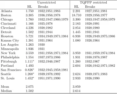
Thus, the results presented in Table 1 point to the best model (either QPPP or TQPPP) for
each series. These results are further categorized as unrestricted (when PPP is not imposed,
second column in Table 1) and restricted (when PPP constraint is imposed on the TQPPP
specification, fourth column in Table 1) models – note that estimated break dates are also
reported.
The estimated HL and the corresponding break points reported in Table 1. As can be seen,
the break points are estimated around the years of the 1929 Great Depression, World War
II4
, the collapse of the Bretton Woods system (1971), the oil shocks (1973, 1979), the great
moderation (mid-eighties), and the early 1990’s economic crisis. These are the major events
affecting the prices in the U.S. and, hence, the prices of U.S. cities, although they have affected
the city price differentials in a heterogeneous way – i.e., note that the break points are not
present in all series.5
Finally, it should be highlighted that some of the estimated break points
are closely in line with the ones detected in Sonora (2009) – he performs the analysis allowing
for a maximum of two structural breaks, which are placed in the Depression era or in the 1970s.
The results concerning HL are very encouraging, with point estimates between one and three
years for majority of the cities. More importantly, the average and median speed of convergence
are not only faster than the estimates obtained by CMS and NS, they are also well below than
Rogoff’s (1996) consensus estimates of 3–5 years. In a simpler setup after allowing for breaks,
Sonora (2009) also obtained faster convergence of city relative prices, while Chen and Devereux
(2003) report a half-life of nearly five years, but did not consider structural breaks in their
analysis. However, the estimates reported in Sonora (2009) and Chen and Devereux (2003) are
not correct unless the model is an AR(1) process, so their conclusions have to be taken with
caution. Our results are not upset when the PPP restriction is imposed in the computation of
HLs. The estimated HLs are within the neighborhood of consensus range: the mean is 3.859 and
the median is 2.614 years. This is reassuring for the different approaches used in the analysis,
as both restricted and unrestricted models show evidence of faster reversion to price level parity
3
Results remain unaffected if we use the Akaike information criterion. A companion appendix containing unreported results is available on request from the corresponding author.
4
The War Production Board and other agencies managed the production and distribution of key fuels and materials. The Office of Price Administration controlled pricing, and basic commodities were rationed. Rationing ended in 1947.
5
in general.
3.2 Half-life Estimates: Pairwise Analysis
The preceding analysis assumes that U.S. city price levels converge towards the aggregate U.S.
price level. The main drawback of this approach is that results can be sensitive to the choice
of the benchmark and, as a result, can lead to misleading conclusions. For example, it could
be that the price deviations between a pair of cities is I(0) stationary, but their deviations
computed separately against the aggregate U.S. price level could be non-stationary. The fact
that price levels converge between this pair would be lost by just focusing on the aggregate U.S.
price level. To overcome this limitation, we follow Pesaran et al. (2009) in order to compute the
pairwise estimates of the price convergence rates. Given N time series of prices, the pairwise
tests focus on all possibleN(N−1)/2 price deviation pairs between the time series in the panel,
and can consistently estimate the proportion of pairs that do not converge.
We have computed median unbiased half-life estimates for all N(N −1)/2 = 136 pairs of
price differentials. In order to get a complete picture, we have summarized in Table 2 the
percentage of HLs that are below, within and above the 3–5 years consensus. Note that the
vast majority of HLs are below or within the consensus for the three different situations that
we consider. Further, Table 2 also reports the mean and median of the HL estimates for the
combination of the QPPP/TQPPP specifications – detailed results for the QPPP and TQPPP
specifications for each pair of time series are available upon request. As can be seen, the median
half-life estimate shows a rapid adjustment to PPP than Rogoff’s (1996) consensus range of 3–5
years, whereas the mean is close to five years. Similar results are also found when using the
QPPP and TQPPP specifications.
4
Conclusions
We have discussed how structural breaks introduce conceptual and econometric difficulties that
complicate the interpretation of PPP, and thereby impacting the computations of the half-life
of PPP deviations. The crux of the issue is that unattended structural breaks introduce an
upward bias in the autoregressive coefficients of the AR models that have been adjusted to
price level differentials. This in turn implies upward bias in the persistence measure of the PPP
deviations, falsely leading us to conclude that shocks affecting price differentials are highly
persistent. Once the structural breaks are accommodated in the analysis, we obtain a median
half-life of convergence ranged between 1.5 and 2.6 years, much faster than those documented in
previous studies. As a check of robustness, we have extended the analysis to conduct pairwise
tests of price level convergence. The finding is broadly consistent with those obtained from
the aggregate U.S. price level. Consequently, our analysis raises a warning flag about common
practice of econometric modeling related to the PPP puzzle.
References
Andrews, D.W.K. and Chen, H.Y. (1994). Approximately median-unbiased estimation of autoregressive models,Journal of Business and Economic Statistics 12, 187-204.
Balassa, B. (1964). The purchasing parity power doctrine: A reappraisal,Journal of Political Economy 72, 584-596.
Basher, S.A. and Carrion-i-Silvestre, J.L. (2009). Price level convergence, purchasing power parity and multiple structural breaks in panel data analysis: An application to U.S. cities,
Journal of Time Series Econometrics 1(1), Article 3.
Cassel, G. (1918). Abnormal deviation in international exchanges, Economic Journal 28, 413-415.
Cecchetti, S.G., Mark, N.C. and Sonora, R.J. (2002). Price index convergence among United States cities, International Economic Review 43, 1081-1099.
Chen, L.L. and Devereux, J. (2003). What can US city price data tell us about purchasing power parity? Journal of International Money and Finance 22, 213-222.
Hamilton, J. D. (1983). Oil and Macroeconomy since World War II, Journal of Political Economy 91, 2, 228-248.
Hansen, B.E. (2001). The new econometrics of structural change: Dating breaks in US labor productivity, Journal of Economic Perspective 15, 117-128.
Nath, H.K. and Sarkar, J. (2009). Unbiased estimation of the half-life to price index conver-gence among US cities,Journal of Money, Credit and Banking 41, 1041-1046.
Perron, P. (1989). The great crash, the oil price shock, and the unit root hypothesis, Econo-metrica 57, 1361-1401.
Pesaran, M.H., Smith, R.P., Yamagata, T. and Hvozdyk L. (2009). Pairwise tests of purchasing power parity,Econometric Reviews 28, 495-521.
Rogoff, K. (1996). The purchasing power parity,Journal of Economic Literature 34, 647-668.
Samuelson, P.A. (1964). Theoretical notes on trade problems,Review of Economics and Statis-tics 46, 145-154.
Table 1: Half-life estimates of price level convergence towards U.S. CPI: QPPP and TQPPP hypotheses specification
Unrestricted TQPPP restricted
HL Breaks HL Breaks
Atlanta 1.750 1932;1951;1983 2.201 1927;1951;1981 Boston 3.305 1936;1956;1978 18.710 1929;1956;1977 Chicago 1.760 1932;1947;1960;1979 3.300 1933;1947;1958;1979 Cincinnati 1.166 1935;1978 2.183 1928;1991
Cleveland 4.226 1938;1982 2.854 1938;1980 Detroit 1.502 1931;1944 1.445 1931;1941
Houston 5.721 1934;1949;1971;1984 6.938 1926;1949;1975;1986 Kansas City 1.381 1931;1964 1.080 1926;1964
Los Angeles 1.263 1930 Minneapolis 1.936 1931
New York 3.559 1931;1958;1971;1984 3.959 1931;1959;1974;1984 Philadelphia 1.554 1937;1973;1986 1.931 1938;1978;1987 Pittsburgh 1.111∗ 1932;1946;1987 1.260 1932;1967
Portland 1.493 2.604 1926;1942;1971;1982 San Francisco 0.826∗ 1932;1945;1958;1981
Seattle 1.268∗ 1939;1978;1992 2.624 1939;1971;1983
St. Louis 1.452∗ 1951;1971;1990 2.933 1926;1990
Mean 2.075 3.859
Median 1.502 2.614
Note: QPPP: Qualified Purchasing Power Parity; TQPPP: Trend Qualified Purchas-ing Power Parity; HL: Half-life. The asterisk behind the HL estimates indicates that the selected specification by BIC information criterion for the corresponding time series is the QPPP one.
Table 2: Proportion of pairwise half-life that are below, within and above the Rogoff’s (1996) 3-5 years consensus view
HL <3 3≤HL≤5 5< HL
QPPP 67.6% 15.4% 16.9% TQPPP 79.7% 6.8% 13.5% Mixed 82.4% 10.3% 7.4%
HL
Mean 5.419 Median 1.766
Note: QPPP: Qualified Purchasing Power Parity; TQPPP: Trend Qualified Purchasing Power Parity. HL: Half-life.