http://dx.doi.org/10.4236/ojs.2016.64055
A New Procedure to Test for Fractional
Integration
William Rea
1, Chris Price
2, Les Oxley
3, Marco Reale
2, Jennifer Brown
21Department of Economics and Finance, University of Canterbury, Christchurch, New Zealand 2Department of Mathematics and Statistics, University of Canterbury, Christchurch, New Zealand 3Waikato Management School, University of Waikato, Hamilton, New Zealand
Received 28 May 2016; accepted 20 August 2016; published 23 August 2016
Copyright © 2016 by authors and Scientific Research Publishing Inc.
This work is licensed under the Creative Commons Attribution International License (CC BY). http://creativecommons.org/licenses/by/4.0/
Abstract
It is now widely recognized that the statistical property of long memory may be due to reasons other than the data generating process being fractionally integrated. We propose a new procedure aimed at distinguishing between a null hypothesis of unifractal fractionally integrated processes and an alternative hypothesis of other processes which display the long memory property. The procedure is based on a pair of empirical, but consistently defined, statistics namely the number of breaks reported by Atheoretical Regression Trees (ART) and the range of the Empirical Fluctu-ation Process (EFP) in the CUSUM test. The new procedure establishes through simulFluctu-ation the bi-variate distribution of the number of breaks reported by ART with the CUSUM range for simulated fractionally integrated series. This bivariate distribution is then used to empirically construct a test which rejects the null hypothesis for a candidate series if its pair of statistics lies on the peri-phery of the bivariate distribution determined from simulation under the null. We apply these methods to the realized volatility series of 16 stocks in the Dow Jones Industrial Average and show that the rejection rate of the null is higher than if either statistic was used as a univariate test.
Keywords
Long-Range Dependence, Strong Dependence, Global Dependence, Regression Trees, CUSUM Test, Volatility
1. Introduction
long memory to refer to fractionally integrated series defined in Section 2 below. A number of other models, apart from fractional integration, have been proposed to account for the extraordinary persistence of the correlations across time found in long memory series, for example; time series with structural change, Markov switching processes, and non-linear processes among others.
The econometrics literature has paid considerable attention to the problem of distinguishing true long memory from structural change in economic or financial time series which exhibit the long memory property because economic and/or financial arguments can be advanced as to why the series studied may have such breaks. For example, [1] confine their study to these two alternatives.
However, the factional integration and structural change models yield significantly different pricing for financial assets, for example see [5] and [6]. Despite the differences in pricing suggested by these authors, the problem of distinguishing between long memory and structural change was reviewed by [1] who suggested “… in the sorts of circumstances studied in this paper, ‘structural change’ and ‘long-memory’ are effectively different labels for the same phenomenon…”.
In light of the substantial literature on long memory vs structural breaks, it would be easy to see our paper as continuing this line of inquiry. However, our purpose is different. The survey of [3] pointed out that in the literature considerable attention has been directed towards understanding the statistical properties of procedures for detecting and quantifying long memory when only structural change is present. On the other hand, the literature on the problem of understanding the statistical properties of procedures for detecting and locating structural change when, in fact, there was only long memory is somewhat sparse. This is primarily because tests for the presence and/or location of structural breaks often report breaks for simulated fractionally integrated series for which the data generating process is uniform throughout. The reporting of multiple breaks where no breaks exist has led most researchers to conclude that structural break methodologies are of no value in dis- tinquishing between true long memory and other processes giving rise to time series which exhibit statistical long memory. In this paper we argue otherwise.
[3] further pointed out that the reason distinguishing between true long memory and the specific alternative of structural breaks is difficult is because their finite sample properties are similar and so standard methodologies fail. Structural break detection and location techniques tend to report breaks when only long memory is present. Indeed, [7] proved that the probability that the standard CUSUM test [8] would report a break in a long memory time series converged to one with increasing series length. Conversely, long memory estimators tend to report estimates of d (defined in Section 2 below) which indicate long memory when only structural breaks are present even in series with memory of only one sample interval.
Nevertheless, efforts have been made to establish tests or procedures which can reliably determine the difference between a true long memory process and ones for which the long memory property arises from some other data generating process. In this literature some significant papers are [9]-[16].
This paper addresses two issues. First, what are the statistical properties of structural break tests when applied to true long memory series? Second, can structural break tests be used to distinquish between true long memory and other processes which give rise to the long memory property. This paper adds to the literature in two ways. We extend the work of [15] to examine, in greater detail, the statistical properties of Atheoretical Regression Trees (ART) [17]-[19] when applied to true long memory processes. It is the essence of the scientific method that a proposed theory or model make clear, testable predictions, and these predictions be tested. Thus our purpose is to test whether the number of breaks reported by ART is consistent or inconsistent with a fractionally integrated data generating process. While it would be preferable to theoretically establish the distribution of reported breaks when ART is applied to fractionally integrated series, it is simple to simulate such series and obtain the required testable prediction, or null distribution, through simulation.
Secondly, by combining two well established empirical structural breaks statistics into a bivariate procedure we show that this bivariate procedure rejects the null hypothesis at a higher rate than either univariate test on its own. The two empirical statistics used are the number of breaks reported by ART and the range of the Cu- mulative Summation (CUSUM) test introduced by [20] and formalised by [8]. As emphasised above the structural breaks methods are being used to obtain the null distribution for a fractionally integrated series and are not being used to either detect or locate structural breaks because under the null hypothesis of true long memory no such breaks exist.
process. For comparison purposes we present the results for univariate tests using ART or CUSUM alone and the results of the recently proposed [16] test for these series.
Stated simply, the essence of our new procedure is to use structural break methods to identify the number of breaks, or the range of the empirical fluctuations process (defined in Section 3 below), in a series and compare that number or range with what we would expect to observe, given the values of d, if the null hypothesis of a fractionally integrated process were generating the data. If the null hypothesis is rejected, all we can conclude is that some alternative process, not that required by the null, is the DGP.
The remainder of this paper is set out as follows. Section 2 gives a brief overview of fractionally integrated series. Section 3 presents the methods used. Section 4 presents the results for distribution of breaks in FI(d) series for univariate ART. Section 5 describes the example data set. Section 6 presents an application to stock market realized volatilities. Section 7 contains the discussion and Section 8 concludes.
2. Models
A number of models have been proposed to account for the extraordinary persistence of the correlations across time found in long memory series. Here we consider fractionally integrated series and series with structural breaks in the mean.
2.1. Fractionally Integrated Series
The most widely used models for long memory series are the Fractional Gaussian Noises (FGNs), a continuous time process, and their discrete time counterparts, the fractionally integrated series of order d. FGNs were introduced into applied statistics by [21] in an attempt to model the exceptionally slow decay in the auto- correlations observed in long memory series. FGNs are the stationary increments of an Gaussian H self-similar stochastic process which we now define.
Definition 1 A real-valued stochastic process
{ }
( )
tZ t
∈ is self-similar with index
H
>
0
if, for anya
>
0
,( )
{
}
{
H( )
}
d
t t
Z at ∈ a Z t
∈
=
where denotes the real numbers and =d denotes equality of the finite dimensional distributions. H is also known as the Hurst parameter.
Definition 2 A real-valued process
{ }
( )
tZ
Z t
∈
=
has stationary increments if, for all h∈R(
)
( )
{
}
d{
( )
( )
0
}
.
t t
Z t
h
Z h
Z t
Z
∈ ∈
+ −
=
−
It follows from Definition 1 that H is constant for all subseries of an H self-similar process.
The stationary increments of an H-self-similar series with
0.5
<
H
<
1
exhibit long memory. It can be shown [22] that the autocorrelations of the increments of an H self-similar process are of the form( )
1(
)
2 2(
)
21 2 1
2
H H H
k k k k
ρ = + − + −
where k≥0 and ρ
( )
k =ρ( )
−k for k<0. Asymptotically( )
(
)
2 2lim 2 1 H .
k ρ k H H k
−
→∞ → −
Thus for 1 2<H<1 the autocorrelations decay so slowly that they are not summable, i.e.
( )
lim . k N N k N k ρ = →∞ =−∑
→ ∞Denoting the backshift operator by B, for a non-integer value of d the operator
(
1
−
B
)
d can be expanded as a Maclaurin series into an infinite order AR representation(
)
(
(
) ( )
)
0
1
1 d
t t k t
k
k d
B X X
k d ∞ − = Γ − − = =
Γ + Γ −
∑
(1)where Γ ⋅
( )
is the gamma function, and t is a innovation term drawn from anN
( )
0,
σ
2 distribution. The operator in Equation (1) can also be inverted and Xt written in an infinite order MA representation. It can be shown [22] that the autocorrelations for a fractionally integrated process are, asymptotically,( )
2d 1k
c k
ρ
−≈
where c is a constant which depends on d, and on any AR(p), and MA(q) components used in the model. For 0< <d 1 2 the autocorrelations decay so slowly that they are not summable. It is this slow rate of decay of the autocorrelations that makes them attractive as models for long memory time series.
The two parameters H and d are related by the simple formula d =H−1 2.
Both FGNs and FI(d) s have been extensively applied as models for long memory time series and their theoretical properties studied. See the volumes by [22] [25][26] and the collections of [27] and [28] and the references therein.
2.2. Constrained Non-Stationary Models
[29] argued that long memory in hydrological time series was a statistical artifact caused by analyzing non- stationary time series with statistical tools which assume stationarity. Often series which display the long memory property are constrained for physical reasons to lie in a bounded range, but beyond that we have no reason to believe that they are stationary. For example, in the series we study in this paper (realized volatilities, see Section 6), as long as the companies remain in the index their stock price volatilities cannot have an unbounded increasing or decreasing trend.
Models of this type which have been proposed typically have stochastic shifts in the mean, but overall are mean reverting about some long term average. The most popular of these are the breaks models which we define as follows:
1
1 i i
p
t t t t i t
i
y I−< ≤ µ
=
=
∑
+ (2)where yt is the observation at time t, It S∈ is an indicator variable which is 1 only if
t
∈
S
and 0 otherwise, tis the time, ti, i=1,,p, are the breakpoints and µi is the mean of the regime i, and t is a noise term. In this case, a regime is defined as the period between breakpoints.
It is important to note that Equation (2) is just a way to represent a sequence of different models (i.e. models subjected to structural breaks). This model only deals with breaks in mean. It can be generalized for any kind of break. In series with a structural break the noise process, t, may also undergo a change. We present this class of model simply by way of example because it has been used by others when studying long memory processes. We do not regard it as the only alternative model to create long memory-like properties.
3. Method
3.1. The Distribution of Breaks Reported by ART
To obtain the null distribution of reported breaks for fractionally integrated series we simulated FI(d) series using farima Sim from the package f Series [30] in R [31] with lengths from 1000 to 16,000 data points in steps of 1000 data points, and d values between 0.02 and 0.48 in steps of 0.02 d units. ART was applied to each series using functions implemented in the tree package of [32] and the number of reported breaks, their locations and associated regime lengths were recorded. For each set of parameter values 1000 replications were run. This yielded a set of 384 simulations which we used as raw data for establishing the mean number of reported breaks and the distributions of those breaks for FI(d) series. The results are reported in Section 4 below.
3.2. The Bivariate Distribution of ART vs CUSUM
We obtained a bivariate distribution of the number of breaks reported by ART [19] and the CUSUM range [8] [20] for FI(d) series under a null hypothesis of true long memory through simulation. ART is an application of standard regression trees [33] to the problem of finding apparent mean shifts in univariate time series. Regression trees are widely used in many branches of statistics but have only infrequently been applied to time series, see [35] for an example. While they have been used to locate structural breaks in time series it must be stressed that we are only using them to obtain the statistic of the reported number of breaks. In the simulated series to which we are applying ART to obtain the reported number of breaks, all breaks are spurious for there are no real breaks in these series. The question of whether the reported breaks in the example data set are structural breaks or something else is not addressed in this paper.
In the CUSUM test the residuals are standardized by dividing by the estimated series standard deviation and the cumulative summation of the residuals is plotted against time. That is
1
1
; 1, ,
ˆ r
r t
t
Z z r T
σ =
=
∑
= where zt is the residual at time t,
σ
ˆ is the estimated standard deviation and T is the length of the time series, is plotted against r. Under a null hypothesis of no structural breaks in the mean (i.e. that the series has a constant local mean), the cumulative summation forms a Brownian Bridge usually referred to as the Empirical Fluctuation Process (EFP). The range of the CUSUM test is simply the difference between the maximum and minimum values of the EFP.This type of method can be usefully thought of as a parametric bootstrap. An important characteristic that is important for our procedure is that the bivariate distributions in later examples shows low correlation between the two statistics (ART and CUSUM). This indicates that the information from the two is complementary, so that the combined test can be expected to perform better than either univariate test on their own.
3.3. The New Procedure
The procedure is as follows and uses several different packages for the R [31] statistical software and comprises the following.
1) Estimate d for the full series. Unless otherwise stated all estimates of d were obtained with the estimator of [35] as implemented in the R package fracdiff of [36].
2) Through simulation, obtain the bivariate probability distribution of number of breaks reported by ART and the CUSUM range for the null distribution of an FI(d) series with d as estimated in the previous step and the same number of observations as the series under test.
a) Simulate a large number of FI(d) series (we used 1000 replications) with appropriate d value and length. FI(d) series were simulated with the function farima Sim in the R package f Series of [30].
b) Use ART to break the series into “regimes” and record the number of reported breaks. c) Obtain the CUSUM range using the efp function in the R package strucchange of [37]. d) Plot the bivariate distribution.
3) Apply ART to the full series to obtain the reported number of break points. 4) Use the efp to obtain the CUSUM range of the full series.
6) Assess whether the bivariate statistic for the series is consistent with the null distribution obtained by simulation. This can be done either visually or by generating contours of significance for the bivariate dis- tribution. Contours of significance can be obtained either by using the data from the simulations or kernel smoothing can be applied if desired.
For comparison purposes we provide the p-values for the univariate ART and CUSUM tests.
4. Univariate ART
[15] determined that the number of breaks reported by ART when applied to Fractional Gaussian Noises was well-described by a Poisson distribution when the series length and the H parameter were fixed. However, his work was quite limited and considered only two series lengths. His work lead to two possible tests based on the number of reported breaks in a long memory series; one using the mean number of reported breaks and the Poisson distribution to determine significance levels; and the other using the simulated data as a bootstrap to estimate the distribution and determine significance levels.
We obtain the mean number of breaks under the null hypothesis of the series being an FI(d) process. If the number of reported breaks in a series under test exceeds the 95% (or other significance) level based on the Poisson distribution then we reject the null of an FI(d) process. It should be noted that [15] interpreted a rejection of the null as indicating the series had structural breaks. However, we do not propose a specific alternative to the null, instead report whether the reported number of breaks is either consistent or inconsistent with the series being fractionally integrated. Alternatively, we obtained sufficient empirical data to establish the 95% confidence interval through simulation.
The method and results presented here are intended to extend his work to obtain a way of gaining a reasonable estimate of the expected number of reported breaks for a wide range of d values and series lengths in fractionally integrated series.
For reasons of space we report a representative selection of results. The remainder are available on request from the authors.
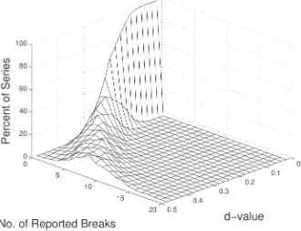
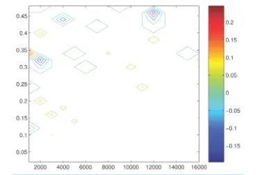
[image:6.595.150.480.442.695.2]The distribution of the number of breaks reported by ART for series with 4000 data points is presented in Figure 1. As [15] noted, as the d parameter increased, the simulated series underwent a transition from ART reporting no breaks to reporting multiple breaks for all replications.
Figure 1. Distribution of the number of breaks reported by ART for 1000 replications of
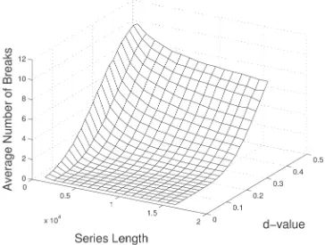
The mean number of reported breaks per series for various series lengths and d values is presented in Figure 2. As can be seen, as the series lengths increased the d values for which no breaks were reported increased. Further, for a fixed d value, the mean number of reported breaks decreased with increasing series length.
We fitted a function to the empirical data to obtain formulas for calculating the mean and various tail probabilities. The approximations are calculated by computing the following variables in the order given:
[
]
23 4
5d x x
γ
++
= − −
2
1 2
q=xγ +xγ
[ ] [ ]
(
)
(
)
(
)
[
] [
] [
]
2 2
7 9 10 5 6 8
2
12 8500 11 2000 0.32 0.46
Q q x q q x d x x x x q
x q x d d
γ γ γ
+ +
+ + +
= + + − + + +
+ − + − − −
[ ]
F= Q+ (3)
( )
floor
f = F (4)
where x1x12 are given in Table 1. The function
[ ]
q + denotes the maximum of q and zero, and similarly for other arguments. The function “floor(z)” returns the greatest integer less than or equal to z. When approximating the mean the step in Equation (4) is omitted; F =[ ]
Q+ is used instead.Each fit has been generated by minimizing a function measuring the error between the fitted function f and the known values y d
( )
, at data points(
d,)
, where d ranges from 0.02 to 0.48 in steps of 0.02, and series length ranges from 1000 to 16,000 in steps of 1000. The minimization is with respect to the parameters1, , 12
x x .
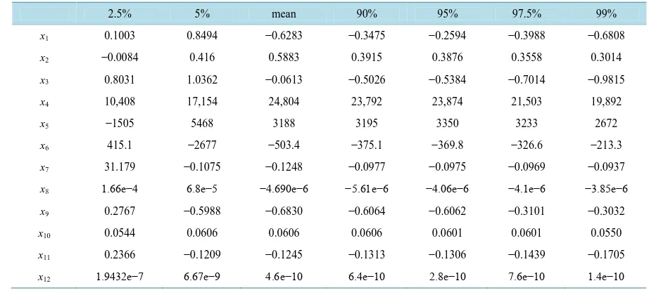
[image:7.595.131.495.416.691.2]The two columns on the left of Table 1 list the parameters for which the probability that the number of breaks is greater than or equal to f is at least 97.5% and 95% respectively. In these cases the relevant error function is given by
Table 1. Coefficients for the function approximating the mean, and various upper and lower quantiles.
2.5% 5% mean 90% 95% 97.5% 99%
x1 0.1003 0.8494 −0.6283 −0.3475 −0.2594 −0.3988 −0.6808
x2 −0.0084 0.416 0.5883 0.3915 0.3876 0.3558 0.3014
x3 0.8031 1.0362 −0.0613 −0.5026 −0.5384 −0.7014 −0.9815
x4 10,408 17,154 24,804 23,792 23,874 21,503 19,892
x5 −1505 5468 3188 3195 3350 3233 2672
x6 415.1 −2677 −503.4 −375.1 −369.8 −326.6 −213.3
x7 31.179 −0.1075 −0.1248 −0.0977 −0.0975 −0.0969 −0.0937
x8 1.66e−4 6.8e−5 −4.690e−6 −5.61e−6 −4.06e−6 −4.1e−6 −3.85e−6
x9 0.2767 −0.5988 −0.6830 −0.6064 −0.6062 −0.3101 −0.3032
x10 0.0544 0.0606 0.0606 0.0606 0.0601 0.0601 0.0550
x11 0.2366 −0.1209 −0.1245 −0.1313 −0.1306 −0.1439 −0.1705
x12 1.9432e−7 6.67e−9 4.6e−10 6.4e−10 2.8e−10 7.6e−10 1.4e−10
( ) ( )
( ) ( )
(
)
2, , 1 , ,
d
F d −y d − ++ F d −y d −
∑∑
(5)
where
[ ]
z − denotes the minimum of z and zero. This error function imposes no penalty when y≤F< +y 1 because the discrete nature of the floor function means f = y. The use of F rather than f in Equation (5) gives a better measure of the fit in the region between data points. The errors with the optimal parameter values for these fits are 0.0332 and 0.0894 respectively.The third column of Table 1 lists the parameter values which gives the fitted approximation to the mean. In this case the least squares error is simply
( ) ( )
(
)
2, ,
d
F d −y d
∑∑
and the approximation is given by F, not f. The residual sum of squares for the optimal fit was 0.4436.
The four columns on the right of Table 1 list the parameters for which the probability that the number of breaks is less than or equal to f is at least 90%, 95%, 97.5% and 99% respectively. For these, the relevant error function is Equation (5). The values of this error function with the optimal parameters are 0.0576, 0.0835, 0.2125, and 0.33 respectively. Clearly the 90% and 95% fits are rather better than the other two. These two fits (90% and 95%) have approximately the same final errors as the two upper quantile fits, however the latter are zero over much larger areas than the 90% and 95% fits. Hence the 90% and 95% fits will have smaller relative errors.
The two upper quantiles given by the first two columns allow two sided tests to be performed. When the lower limit on the two sided test is zero, the lower limit effectively says nothing as the number of breaks can not be negative. In such cases a one sided test should be used in place of the two sided test.
Figure 3 presents the differences between the fitted functions estimated upper 95 percent confidence interval and that estimated from the empirical data.
5. The Data Set
Figure 3. Errors in the fitted function to the empirically determined 95 percent confidence intervals using the formulas in the text. The horizontal axis is the series length, the vertical axis is the d value used in the simulations.
five-minute grids, which is a consistent estimator of the daily volatility. A fuller explanation of the dataset and how the realized volatilities were calculated can be found in [38]. It should be noted that all 16 stocks were major American corporations traded on the New York Stock Exchange. They are subject to correlated shocks and so cannot be considered to be independent series.
6. Application-Realized Volatilities
We applied the bivariate ART vs CUSUM range as described in the Section 3 to the 16 series in the data set. For reasons of space we present only a representative selection of results, the remainder are available on request from the authors. The four results from the new computational procedure are presented for series with d
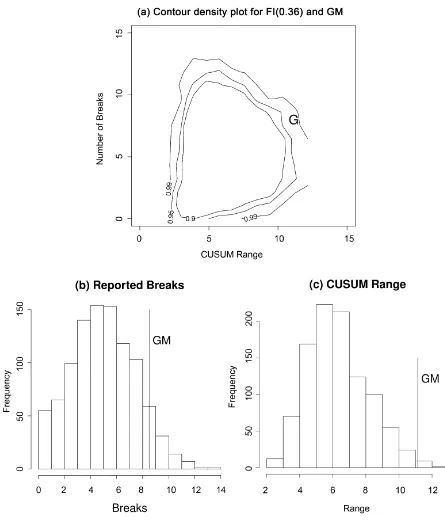
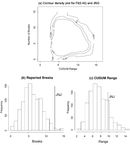
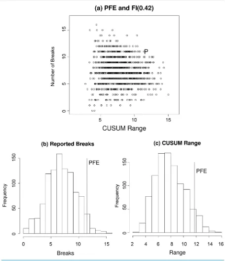
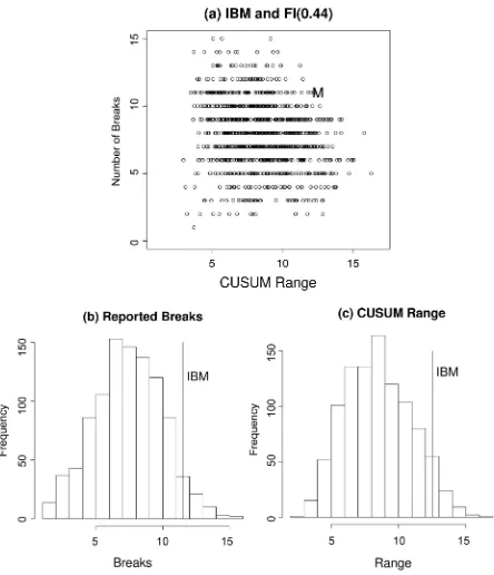
estimates of 0.36 (GM), 0.40 (JNJ), 0.42 (PFE), and 0.44 (IBM) in panel (a) of Figures 4-7. For comparison purposes we plot the corresponding univariate results for the reported number of breaks and the CUSUM range in panels (b) and (c) respectively. These four results include one example for which the null can be rejected by univariate ART (JNJ), one by univariate CUSUM (GM), and two (IBM, PFE) for which the null is not rejected by either univariate test but is rejected by the bivariate procedure.
In Figures 4-7 the vertical axis is the number of breaks reported by ART. When considered as a discrete univariate distribution the vertical axis is simply the test of [15]. We provide the results of the Zheng test for all series in the column labelled “ART Test p-value” in Table 2 below. As can be seen from the table the null hypothesis of true long memory was only rejected for one of the 16 series at the five percent level, a result which could easily have occurred by chance. With the exception of Johnson and Johnson, JNJ, (see Figure 5) the number of reported breaks in these series was not in the tails of the univariate distribution. Thus the null hypothesis of a fractionally integrated series would not be rejected on the basis of Zheng’s univariate test.
Figure 4. (a) Bivariate distribution of the CUSUM range and number of breaks reported by ART for 1000 replications of in an FI(0.36) series of 2539 data points. The letter “G” denotes the GM data point. (b) and (c) are the corresponding univariate
distributions for the number of reported breaks and the CUSUM range respectively.
the exception was Walmart (WMT).
To summarise, the results of univariate ART and CUSUM tests are presented in columns “ART Test p-value” and “CUSUM Test p-value” respectively in Table 2. As can be seen the null of true long memory was rejected for 1 of the 16 series by the univariate ART test and for 12 of the 16 series by the univariate CUSUM test.
Figure 5. Distribution of the number of breaks reported by ART for 1000 replications of an FI(0.40) series of 2539 data points. The letter “J” denotes the JNJ data point. (b) and (c) are the corresponding univariate distributions for the number of
reported breaks and the CUSUM range respectively.
correlations and well understood asymptotic properties which allowed them to theoretically derive critical values for varying levels of statistical significance. The results of their test are presented in the column labelled “ORT” of Table 2. The null of true long memory was rejected for one of the 16 series at the five percent level, a result which could easily have occurred by chance.
7. Discussion
Figure 6. Distribution of the number of breaks reported by ART for 1000 replications of an FI(0.42) series of 2539 data points. The letter “P” denotes the PFE data point. (b) and (c) are the corresponding univariate distributions for the number of reported breaks and the CUSUM range respectively.
which display apparent long memory properties is difficult. This paper’s primary contribution is that we present a procedure based on the use of a bivariate distribution which, in the 16 series examined, appears to easily show the realized volatility 15 of the series are not FI(d). Secondarily we have extended the work of [15] on univariate ART.
Figure 7. (a) Bivariate distribution of the CUSUM range and number of breaks reported by ART for 1000 replications of FI(0.44) series of 2539 data points. The letter “M” denotes the IBM data point. (b) and (c) are the corresponding univariate
distributions for the number of reported breaks and the CUSUM range respectively.
Table 2. For the 16 stocks, the d estimate is that reported by the estimator of [35]. The actual and expected breaks reported by ART, together with p-values calculated from Poisson Distribution as in the [15] test. The column “CUSUM Test p-value” is the p-value for the univariate CUSUM test with critical values obtained by simulation. Results for which the null is rejected at at least the five percent level are marked by an asterisk (*). The final column lists the test statistic for the [16] test.
Those results for which the null is rejected at at least the five percent level are marked by an asterisk (*).
Reported Expected ART Test CUSUM ORT
Series d Est Breaks Breaks p-value Test p-value
AA 0.42 7 7.5 0.48 *0.00 2.68
AIG 0.40 6 6.8 0.52 *0.00 4.02
BA 0.40 10 6.8 0.09 *0.01 1.63
CAT 0.41 7 7.1 0.42 *0.01 5.32
GE 0.44 8 8.0 0.41 *0.01 4.98
GM 0.36 7 5.5 0.19 *0.01 5.20
HP 0.44 6 8.0 0.69 *0.00 0.50
IBM 0.44 11 8.0 0.11 0.06 1.13
INTC 0.46 6 8.6 0.75 *0.00 2.20
JNJ 0.40 11 6.8 *0.05 0.16 3.62
KO 0.42 11 7.5 0.08 *0.00 4.40
MRK 0.39 7 6.4 0.31 *0.05 3.89
MSFT 0.46 10 8.6 0.25 *0.03 *11.24
PFE 0.42 10 7.5 0.14 0.07 3.88
WMT 0.42 10 7.5 0.14 0.31 4.15
XON 0.44 6 8.0 0.69 *0.00 1.26
The results reported by [15] were encouraging but our results with realised volatilities, reported in Table 2, indicated that the problem of the finite sample properties of FI(d) series and series with structural breaks being similar rendered the test of little help in practice.
With the exception of the [9] test, tests based on univariate distributions have, in general, not been successful in distinguishing among the proposed models. The results of the [16] test had the same rate of rejection of the null as the [15] test. The simple CUSUM test with null distributions obtained by simulation rejected the null of true long memory at a much higher rate than either the [15] or the [16] test.
The results of looking at the data with a bivariate breaks vs CUSUM range distribution, as in Figures 4-7, are promising and we believe points the way for future progress in this area. On these bivariate distributions the data point for each of the four real time series was clearly in the extremes of the tails of the distribution. Indeed, all four of the results presented here appear to be significant at close to the 0.001 level. Of the 16 series, 15 of them were unable to accept the null hypothesis of an FI(d) series with d as estimated for the full series.
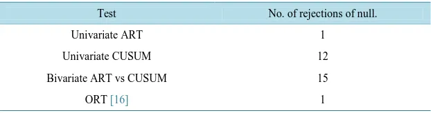
A summary of the results for all four tests and procedures is presented in Table 3.
8. Conclusions and Future Research
Table 3. A summary of the number of rejections of the null by test or procedure.
Test No. of rejections of null.
Univariate ART 1
Univariate CUSUM 12
Bivariate ART vs CUSUM 15
ORT [16] 1
15 of the 16 series. This is a higher rate of rejection than using either of the two statistics, which form the bivariate distribution, in their univariate forms seperately.
There are unresolved statistical issues which merit further research. In the bivariate approach we have estimated d but then proceeded as if the d value was known a priori. Clearly the bivariate distribution is dependent on d and further work needs to be done to establish the usefulness of the approach. Also tests of other models which display the long memory property need to be carried out.
Finally, it must be stressed that this new procedure uses the number of breaks to ascertain whether the series is likely to be generated by a fractionally integrated prcoess. In rejecting the null we do not conclude that the alternative is actually a breaks model. There may be possible alternatives to the null and our procedure is simply to test for fractional integration.
Acknowledgements
We would like to thank the participants in the MODSIM09 conference and two anonymous referees for helpful and constructive feedback.
References
[1] Diebold, F.X. and Inoue, A. (2001) Long Memory and Regime Switching. Journal of Econometrics, 105, 131-159.
http://dx.doi.org/10.1016/S0304-4076(01)00073-2
[2] Granger, C.W.J. and Hyung, N. (2004) Occasional Structural Breaks and Long Memory with an Application to the S&P 500 Absolute Stock Returns. Journal of Empirical Finance, 11, 213-228.
http://dx.doi.org/10.1016/j.jempfin.2003.03.001
[3] Sibbertsen, P. (2004) Long Memory versus Structural Breaks: An Overview. Statistical Papers, 45, 465-515.
http://dx.doi.org/10.1007/BF02760564
[4] Banerjee, A. and Urga, G. (2005) Modelling Structural Breaks, Long Memory and Stock Market Volatility: An Over-view. Journal of Econometrics, 129, 1-34. http://dx.doi.org/10.1016/j.jeconom.2004.09.001
[5] Bollerslev, T. and Mikkelson, H. (1996) Modeling and Pricing Long Memory in Stock Marker Volatility. Journal of Econometrics, 73, 151-184. http://dx.doi.org/10.1016/0304-4076(95)01736-4
[6] Taylor, S.J. (2000) Consequences for Option Pricing of a Long Memory in Volatility. Mimeo. In: Lee, C.-F. and Lee, J., Eds., Handbook of Financial Econometrics and Statistics, Springer Science + Business Media, New York, 903-932.
http://dx.doi.org/10.1007/978-1-4614-7750-1_32
[7] Wright, J.H. (1998) Testing for a Structural Break at Unknown Date with Long-Memory Disturbances. Journal of Time Series Analysis, 19, 369-376. http://dx.doi.org/10.1111/1467-9892.00097
[8] Brown, R.L., Durbin, J. and Evans, J. (1975) Techniques for Testing the Constancy of Regression Relationships over Time. Journal of the Royal Statistical Society Series B, 37, 149-192.
[9] Beran, J. (1992) A Goodness-of-Fit Test for Time Series with Long Range Dependence. Journal of the Royal Statistic-al Society B, 54, 749-760.
[10] Beran, J. and Terrin, N. (1996) Testing for a Change in the Long-Memory Parameter. Biometrika, 83, 627-638.
http://dx.doi.org/10.1093/biomet/83.3.627
[11] Beran, J. and Terrin, N. (1999) Testing for a Change in the Long-Memory Parameter. Biometrika, 86, 233.
http://dx.doi.org/10.1093/biomet/86.1.233
[12] Teverovsky, V. and Taqqu, M. (1999) Testing for Long-Range Dependence in the Presence of Shifting Means or a Slowly Declining Trend, Using a Variance-Type Estimator. Journal of Time Series Analysis, 18, 279-304.
[13] Smith, A.D. (2005) Level Shifts and the Illusion of Long Memory in Economic Time Series. Journal of Business and Economic Statistics, 23, 321-335. http://dx.doi.org/10.1198/073500104000000280
[14] Berkes, I., Horvath, L. and Kokoszka, P. (2006) On Discriminating between Long-Range Dependence and Changes in Mean. The Annals of Statistics, 34, 1140-1165. http://dx.doi.org/10.1214/009053606000000254
[15] Zheng, G.Y. (2007) The Distributions of Change Points in Long Memory Processes. In: Oxley, L. and Kulasiri, D., Eds., MODSIM 2007 International Congress on Modelling and Simulation, Modelling and Simulation Society of Aus-tralia and New Zealand, 3037-3043.
[16] Ohanissian, A., Russell, J.R. and Tsay, R.S. (2008) True or Spurious Long-Memory? A New Test. Journal of Business and Economic Statistics, 26, 161-175. http://dx.doi.org/10.1198/073500107000000340
[17] Rea, W., Reale, M., Cappelli, C. and Brown, J. (2006) Identification of Level Shifts in Stationary Processes. In Newton, J., Ed., Proceedings of the 21st International Workshop on Statistical Modeling, Galway, 3-7 July 2006, 438-441. [18] Cappelli, C., Penny, R.N., Rea, W.S. and Reale, M. (2008) Detecting Multiple Mean Breaks at Unknown Points with
Atheoretical Regression Trees. Mathematics and Computers in Simulation, 78, 351-356.
http://dx.doi.org/10.1016/j.matcom.2008.01.041
[19] Rea, W.S., Reale, M., Cappelli, C. and Brown, J. (2010) Identification of Changes in Mean with Regression Trees: An Application to Market Research. Econometric Reviews, 29, 754-777. http://dx.doi.org/10.1080/07474938.2010.482001
[20] Page, E.S. (1954) Continuous Inspection Schemes. Biometrika, 41, 100-115.
http://dx.doi.org/10.1093/biomet/41.1-2.100
[21] Mandelbrot, B.B. and van Ness, J.W. (1968) Fractional Brownian Motions, Fractional Noises and Applications. SIAM Review, 10, 422-437. http://dx.doi.org/10.1137/1010093
[22] Beran, J. (1994) Statistics for Long Memory Processes. CRC Press, Boca Raton.
[23] Granger, C.W.J. and Joyeux, R. (1980) An Introduction to Long-Range Time Series Models and Fractional Differenc-ing. Journal of Time Series Analysis, 1, 15-29. http://dx.doi.org/10.1111/j.1467-9892.1980.tb00297.x
[24] Hosking, J.R.M. (1981) Fractional Differencing. Biometrika, 68, 165-176. http://dx.doi.org/10.1093/biomet/68.1.165
[25] Embrechts, P. and Maejima, M. (2002) Selfsimilar Processes. Princeton University Press, Princeton. [26] Palma, W. (2007) Long-Memory Time Series Theory and Methods. Wiley-Interscience, Hoboken.
[27] Doukhan, P., Oppenheim, G. and Taqqu, M. (2003) Theory and Applications of Long-Range Dependence. Birkhaüser, Basel.
[28] Robinson, P.M. (2003) Time Series with Long Memory. Oxford University Press, Oxford. [29] Klemes, V. (1974) The Hurst Phenomenon—A Puzzle? Water Resources Research, 10, 675-688.
http://dx.doi.org/10.1029/WR010i004p00675
[30] Wuertz, D. (2005) FSeries: Financial Software Collection. R Package Version 220.10063.
[31] R Development Core Team (2005) R: A Language and Environment for Statistical Computing. R Foundation for Sta-tistical Computing, Vienna, Austria.
[32] Ipley, B. (2005) Tree: Classification and Regression Trees. R Package Version 1.0-19.
[33] Breiman, L., Friedman, J., Olshen, R. and Stone, C. (1993) Classification and Regression Trees. CRC Press, Boca Ra-ton.
[34] Cooper, S.J. (1998) Multiple Regimes in US Output Fluctuations. Journal of Business and Economic Statistics, 16, 92- 100.
[35] Haslett, J. and Raftery, A.E. (1989) Space-Time Modelling with Long-Memory Dependence: Assessing Ireland’s Wind Power Resource. Applied Statistics, 38, 1-50. http://dx.doi.org/10.2307/2347679
[36] Fraley, C., Leisch, F., Maechler, M., Reisen, V. and Lemonte, A. (2006) Fracdiff: Fractionally Differenced ARIMA Aka ARFIMA (p, d, q) Models. R Package Version 1.3-0.
[37] Zeileis, A., Leisch, F., Hornik, K. and Kleiber, C. (2002) Strucchange: An R Package for Testing for Structural Change in Linear Regression Models. Journal of Statistical Software, 7, 1-38. http://dx.doi.org/10.18637/jss.v007.i02
[38] Scharth, M. and Medeiros, M.C. (2009) Asymmetric Effects and Long Memory in the Volatility of Dow Jones Stocks. International Journal of Forecasting, 25, 304-327. http://dx.doi.org/10.1016/j.ijforecast.2009.01.008
[39] Zhang, L., Mykland, P. and Aït-Sahalia, Y. (2005) A Tale of Two Time Scales: Determining Integrated Volatility with Noisy High-Frequency Date. Journal of American Statistical Association, 100, 1394-1411.
http://dx.doi.org/10.1198/016214505000000169
Submit or recommend next manuscript to SCIRP and we will provide best service for you: Accepting pre-submission inquiries through Email, Facebook, LinkedIn, Twitter, etc.
A wide selection of journals (inclusive of 9 subjects, more than 200 journals) Providing 24-hour high-quality service
User-friendly online submission system Fair and swift peer-review system
Efficient typesetting and proofreading procedure
Display of the result of downloads and visits, as well as the number of cited articles Maximum dissemination of your research work
![Table 2. For the 16 stocks, the d estimate is that reported by the estimator of [35]. The actual and expected breaks reported by ART, together with p-values calculated from Poisson Distribution as in the [15] test](https://thumb-us.123doks.com/thumbv2/123dok_us/7874024.739025/14.595.89.537.141.425/estimate-reported-estimator-expected-reported-calculated-poisson-distribution.webp)