General Concave Integral Control

(1)

http://dx.doi.org/10.4236/ica.2013.44042

General Concave Integral Control

Baishun Liu, Xiangqian Luo, Jianhui Li

Academy of Naval Submarine, Qingdao, China

Email: [email protected], E-mail: [email protected], E-mail: [email protected]

Received September 6,2013; revised October 6, 2013; accepted October 13, 2013

Copyright © 2013 Baishun Liu et al. This is an open access article distributed under the Creative Commons Attribution License, which permits unrestricted use, distribution, and reproduction in any medium, provided the original work is properly cited.

ABSTRACT

In this paper, a class of fire-new general integral control, named general concave integral control, is proposed. It is de- rived by normalizing the bounded integral control action and concave function gain integrator, introducing the partial derivative of Lyapunov function into the integrator and originating a class of new strategy to transform ordinary control into general integral control. By using Lyapunov method along with LaSalle’s invariance principle, the theorem to ensure regionally as well as semi-globally asymptotic stability is established only by some bounded information. More- over, the highlight point of this integral control strategy is that the integrator output could tend to infinity but the integral control action is finite. Therefore, a simple and ingenious method to design general integral control is founded. Simulation results showed that under the normal and perturbed cases, the optimum response in the whole domain of interest can all be achieved by a set of the same control gains, even under the case that the payload is changed abruptly. Keywords: General Integral Control; Nonlinear Control; Nonlinear integrator; Concave Function Gain Integrator;

Bounded Integral Control Action; Output Regulation

1. Introduction

Integral control [1] plays an important role in control system design because it ensures asymptotic tracking and disturbance rejection. In the presence of the parametric uncertainties and unknown constant disturbances, integral control can still preserve the stability of the closed- loop system and create an equilibrium point at which the tracking error is zero. The main task of the integral controller is to stabilize this point, which is challenging because it depends on uncertain parameters and unknown disturbances.

1.1. Classical Integral Control

The simplest controllers that achieve integral action are of the proportional integral derivative (PID) form that introduces integral action by integrating the error. It is well known that integral-action controllers with this class of integrator often suffer a serious loss of performance due to integrator windup, which occurs when the actua- tors in the control loop saturate. Actuator saturation not only deteriorates the control performance, causing large overshoot and large settling time, but can also lead to instability, since the feedback loop is broken for such saturation. To disguise this drawback, various anti-

(2)

into the integrator. All these integrators, except for the one proposed by [7], were designed by using the error as the indispensable element. So, all of them is called classical integral control.

1.2. General Integral Control

In 2009, general integral control, which uses all available state variables to design the integrator, is originated in [17], where presents a unified framework for general integral control, some general integrator and controller, the necessary conditions and basic principles for design- ing a general integrator, however, their justification was not verified by strictly mathematical analysis. In 2012, based on linear system theory, we present a systematic design method for general integral control [18] with a linear integrator on all the state of dynamics. The results, however, were local. The regionally as well as semiglobally results were proposed in [19], where presents a nonlinear integrator shaped by sliding mode manifold, and then general integral control design is achieved by sliding mode technique and linear system theory. Therein, the sprout of concave function gain integrator appeared. In 2013, based on feedback linearization technique, a class of nonlinear integrator which is shaped by diffeo- morphism, and a systematic design method for general integral control are presented by [20] and the conditions to ensure regionally as well as semiglobally asymptotic stability are provided.

This paper is not a simple extension of the work [19], but it is developed as a class of fire-new general integral control, named general concave integral control in such a way of normalization. The main contributions are as follows: 1) the partial derivative of a class of general Lyapunov function is firstly introduced into the integrator design; 2) the bounded integral control action and concave function gain integrator are normalized; 3) a general strategy to transform ordinary control into general integral control is proposed; iv) by using Lyapunov method and LaSalle’s invariance principle, the theorem to ensure regionally as well as semi-globally asymptotic stability is established only by some bounded information. Moreover, the highlight point of this integral control strategy is that the integrator output could tend to infinity but the integral control action is finite. Therefore, a simple and ingenious method to design general integral control is founded.

Throughout this paper, we use the notation m

 

A

and M

 

A to indicate the smallest and largest eigen-

values, respectively, of a symmetric positive define bounded matrix A x

 

, for any xRn. The norm of vector x is defined as x  x xT , and that of matrix

A is defined as the corresponding induced norm

 

T M

The remainder of the paper is organized as follows: Section 2 describes the system under consideration, assumption, and definition. Section 3 addresses the control design. Simulation is provided in Section 4. Con- clusions are presented in Section 5.

2. Problem Formulation

Consider the following nonlinear system,











,,



, x f x w g x w u

y h x w

  

   



(1)

where _x_Rn

m

is the state, _u_Rm is the control input, yR is the controlled output, is a vector of unknown constant parameter and disturbance. The functions

l

wR



,



f x w , g x w



,



and are continuous

in



h x,w





x w u, ,



x u Dw

on the domain

n m R R _Rl

D D     . In this study, the function



,



f x w does not necessarily vanish at the origin; i.e.,



0,



0

f w  . Let be a vector of constant

reference. Set

m R r rD 



,w



 _v

v r and _v _r _w. We

want to design a feedback control law such that D

 D D D

u

 

y t r as t .

Assumption 1: For each v, there is a unique

pair

vD



x u0, 0



that depends continuously on and satisfies the equations,

v













0 0

0

0 , ,

,

f x w g x w u

y r h x w

  

    

0₍₂₎

so that x0 is the desired equilibrium point and 0 is

the steady-state control that is needed to maintain equilibrium at

u

0

x , where yr.

For convenience, we state all definitions, assumptions and theorems for the case when the equilibrium point is at the origin of , that is, 0 . There is no loss of

generality in doing so because any equilibrium point can be shifted to the origin via a change of variables.

n

R x 0

Assumption 2: No loss of generality, suppose that the function g x w



,



satisfies,



,



0 0, w, x

g x w g   w D  x D (3)



,

 

0,



x , ,

g w x

g x w g w l x  w D  x D . (4) where x

g

l is a positive constant.

Assumption 3: Suppose that thereexists a control law

 

x

u x such that x0 is an exponentially stable equilibrium point of the system,



,





0,





,

 

x



x f x w  f w g x w u x (5) and there exists a Lyapunov function that satis-

fies, x

 

V x

 

2

1 x

c x V x c x2 2 (6)

(3)

         





2 3

, 0, ,

x

x V x

f x w f w g x w u x c x

x



   



(7)

 

4 x

V x

c x x





 (8)

for all xDx, r and w. Where , ,

and c are all positive constants.

rD wD c₁ c₂

3

c ₄

For the purpose of this note, we introduce the follow-ing definition and property, which is proposed by [13].

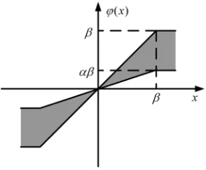
Definition 1: F



 , ,x



with 1  0 ,  0

and n

xR denotes the set of all continuous differential increasing bounded functions,

 

T

1 1 2 2 n n

x x x x

 _{ }    _ such that

 

x   x  x  x R x: 

 

x

    x R x: 

 

[image:3.595.99.246.596.717.2]

1 d  x dx0  x R where  stands for the absolute value.

Figure 1 depicts the region allowed for all the functions belonging to function set F



 , ,x



. For instance, the hyperbolic tangent, arc tangent functions and so on.

An important property of function 

 

x elonging to function set

b





, ,

F   x is that the Euclidean norm of

 

x

 satisfies for all n

xR ,

 

x n

  (9)

3. Control Design

For achieving asymptotic regulation and disturbance rejection, we need to include “integral action” in the control law u. Thus, general integral controller are proposed as follows,

 





1

 

d d

x T

x

u u x K

V x x

 

    

  

 

 

  (10)

where i



d i

 

i di



1 Vx

 

x xi i1, 2, , m



 

 , ;

Figure 1. F



α β, ,x



 

 

functions.

belongs to function set F



 , ,x



. K_ is a positive define diagonal m m m

Thus, substituting (10) into (1) to m

atrix.

obtain the aug-ented system,







   



 

,

 

x f x w , _x ,

T

x

g x w u x g x w K

V x x

   



 _{ } _

 (11)

By Assumption 1 and choosing

  



K_ x

to be nonsingular and large enough, and then set 0 and x0 of

the Equation (11), we obtain,



0,



 

0



0,



g w K_   f w (12) Therefore, we ensure that there is a unique solution

0

 , and then



0,₀



is a unique equilibrium point of closed-loop (11) in the control domain of interest. At the equilibrium point, yr, irrespective of the value of w.

Now, the design task is to provide the conditions on th

the system

e positive constants c₃, c₄ and matrix K_ such that



0,0



is an asympto all stable equilibrium point of the closed-loop system (11) in the control domain of interest, which is not a trivial task because the closed-loop system depends on the unknown vector w. This is established in the following theorem.

Theorem 1: Under Assumptions 1-3, if there exists a po

tic y

sitive define diagonal matrix K_ such that the the following inequalities,

 



0







m g K 0,w

    f (13)

3 4

x g

c c l  m K_ hold, and then

(14)



0,0



clo

is an exponentially stable equilibrium point of the sed-loop system (11). Moreover, if all assumptions hold globally, and then it is globally exponentially stable.

Proof: To carry out the stability analysis, we consider the following Lyapunov function candidate,

   





 

   











   



0

0 0

, x

V x    V x

0, 2

T

g w K_

       

   (15)

Obviously, Lyapunov function candidate (15) is positive define. Therefore, our task is to show that its time derivative along the trajectories of the closed-loop system (11) is negative define, which is given by,

 





 

  





 



           





   



   



0

,

V x   

0,

, , ,

0,

T x

x

V x g w K

V x

f x w g x w u x g x w K x

V x

g w K

x



     

 

   

  



  

 

 



 _

(16)

(4)

Substituting (12) into (16), we obtain,

   





         



 















 

   



 



   



 



0

0,

0

,

, 0, ,

, 0,

0,

x

x V x

V x

f x w f w g x w u x x

V x

g x w g w K

x V x

V x

g w K

x



    

 

   

 

  

 

 

 

 



 

 

(17)

Using (4), (7), (8) and (9), we get,

g w K

x 



 





         





     





 





0

2 2

3 4

,

, 0, ,

, 0,

x

x g

V x

V x

2

3 4

x g

f x w f w g x w u x x

V x

g x w g w K

x

c x c l m K x



    

 



 

  

 

 



  



(18)

Using the fact that Lyapunov function candidate (15) is a positive define function and its time derivative is a negative define function if the inequalities (13) and (14) hold, we conclude that the closed-loop system (11) is stable. In fact, means and

c c l  m K_ x

  

0

V x0   ₀. By

invoking LaSa riance p to

know that the closed-loop system (11) is exponentially stable.

Corollary 1: If the function

lle’s inva rinciple [21], it is easy



,



g x w is equal to a constant, and then the integrator can be taken as

 





1

 

d d

T

x

V x x

        or T

 

x

V x x

    . Thus, under Assumptions 1 and 3, we only need to choose the gain matrix K_ to be nonsingular and large enough such tha inequality (13) holds, and then



0, 0



t the

 is an exponentially stable equilibrium point of the closed-loop system (11). Moreover, if all assumptions hold globally, and then it is globally exponentially stable.

Th gumen

Discussion 1: compared with tegral control pro

tion be

e proof can follow the similar ar t and procedure. It is omitted because of the limited space.

the in -

posed by [19], the main differences are as follows: 1) the integral control action is not confined to the hyperbolic tangent function and can be taken as any func- longing to function set F



 , ,x



, and then the normalization of integral control action is achieved;

2) the indispensable element of integrator is not confined to sliding mode manifold and can be taken as the partial derivative of any Lyapunov function, which satis- fie

o th

is not co

atis- fie

s Assumption 3, and then not only the normalization of concave function gain integrator is achieved but als

e partial derivative of Lyapunov function firstly is introduced into the integrator design.

3) the control element ux



x nfined to slid-

ing control and can be taken as any control, which s



s the conditions of Assumption 3.

Remark 1: The proof of Theorem 1 seems to be very simple, in fact that is not the case because there are two tedious troubles to be concealed in the stability analysis, one is that integral control action must be bounded, an- other is how cancel the terms on  

 

 

 

0 .

There-fore, for solving these two troubles above, an ingenious design method is proposed as follows: just the integrator is taken as T



d

 

d



1

 

x

V x x

        , which is

obtained by differentiating the function  

 

and us-ing the partial derivative of Lyapunov function

 

x

V x x

  as the indispensable element of integrator, and then we get T

 

x

V x x

     . Thus, we not only obtain a bounded integral control action K_ 

 

but also cancel the terms on  

 



 

0 time

de-rivative of Lyapunov function, and then Theorem 1 can be established only by some bounded information.

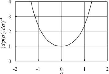
Con-sequently, the ve integral

control is verified. Moreover, this resulte new integrator with a concave function gain

 

 

on of general c in the

onca d justificati

in a class of





1

d  d  , 2. This is why the control law (10) is called general concave i

Remark 2: From the control law (10), vious that the highlight point of thi ontrol strategy is that the integrator output could tend to infinity but the integral control action is finite, which is the same as the one proposed by [19]. This means that this kind of integral control can devote its mind to counteract the unknown constant uncertainties or disturbances and filter out the other action, and then the stability analysis is easy to be achieved in theory and actua

see Figure

ntegral control.

it is ob s integral c

tor saturation is easy to be eliminated in practice.

Remark 3: From the statement above, it is easy to see that: for achieving the integral control, we only need to find a control input ux

 

x and a Lyapunov function

 

x

[image:4.595.332.510.597.718.2]

V x such that x0 is an exponentially stable equilibrium point of the system (5). Especially, when the

(5)

function g x w



,



condition (14) can be on the closed

(13), is th

results in a class control int

, that is, m ed into general oreover, t and Vx

 

x

he mo

is equal to a constant, the dilemma removed, that is, the stable condi-tions -loop system (11), except for the con-dition e same as the one of the system (5). This not only of general strategy to transform ordinary o general integral control but also the guess [17] any control laws can easily be transform integral control laws, is verified partly. M here is great freedom in the choice of

such that the control engineers can st appropriate control input

 

x u x

choose t ux

 

x

r. in on thes

hand to design their own general integral controlle

Based e statements above, it is not hard to know that all of them constitute a simple and ingenious method to design general integral control together.

4. Simulation

Consider the pendulum system [21] described by,

sin

a b cT

   

where ag l0, bk m0, c1 ml2 0,  is gle sub d by the rod and the vertical axis, and T is the torque applied to the pendulum. Vie as the control input and suppose we want to regulate

the an tende

w T  to  . Taking x1   , x2  and uT , the pendu-

lum system can be written as,





1 2 1 2 sin x x 2

x a x

  

  bx c

 

   u (19) point

is and



It is easily to know that the desired equilibrium





T

0 0 0

x  u0 asin

 

 c is the steady-

to maintain equilibrium at

state control that is needed x0.

Thus, t tio as,

 

1 1 2 2

x

u x  k x k x , where k1 and k2 are all positive

nstants.

Substituting ux

 

x into (19) and deleting the

con-ant term

he control law in Assump n 3 can be taken

st co

 

cos

a 

 Linear n of the

sys-tem about the origin, we obtain

, and then izatio ,

x Ax (20) where

 









 of 1 0 1 

 cos 2

A

a  ck b ck

 _ _ _{ } 



Now, using the linear system theory, the choice

 

1 cos

k  a  c and k₂0 ensures that the matrix A e parameter perturbations on a0, 0, 0

b c

is Hurwitz for all th and all

,  



 ,



apunov ov functio

x. Thus,

, and then x = able e

r any gi

itive define atisfied L

e Lyapun Assu

ng

0 is an

symmetric 3 can be ex

o matrix P that s taken as V x

ponentially st quilibrium point of the system (20). Therefore, f ven positive define symmetric ma-trix Q there exists a unique pos

y

n in

P taki

equation T

PAA P Q,

and then th mption

 

T

x

   tanh

 

 ,

 

tanh 1

  ,  1 and choosing k_ , s ch that u

 

sin

 

ck_  a  holds for all a > 0, c > 0 and



π,π



 

co

, and then a globally exponentially stable ntroller can be given as,





 

1 1 2 2





2

21 22 2

, tanh

cosh

u x k x k x k

p p x

             

By taking k1 8



p x12 1





 , k23, k 10, a10, b1, and c10, and then solving the Lyapunov equation

T

PAA P Q, we obtain,

12 21 22 38 1 1 0 p p p          140 0 0 4.2 Q 11 .1 P p _    where     

  a

0 1

 

nd

al parame

31 A   _

70  ters are

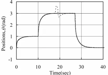
In simulation, the norm a c 10

and b1. In to 0.5 and 5, the

the pe espectively

rturbed case,

, co ponb din d and c

to

are reduced oubling of

pulse

r rres g

mass. Moreover, we consider an additive im - like disturbance d t

 

of magnitude 60 acting on the

[image:5.595.320.526.562.705.2]

ween 18 s an system input

Figure 3 (solid line) a lowing obser ed case n control gain changed abru ca b n r v p et

showed the sim d pertu ations

s, the o terest can all be ac

s, even un ptly

d 19

ulation under normal bed (dashed lin ses. The fol- can be made: und e normal and timum response the whole do- hieved by t of the same d case that the payload is . This demonstr general con- st conver s. results e) c er th in a se ates that a perturb

main of i

er the

ve integral control has strong robustness, fa - gence and good flexibility and can effectively deal with unknown exogenous disturbances, nonlinearity and uncertainties of dynamics.

5. Conclusions

A class of fire-new general integral control named gen-

Figure 3. Sy turbed case (d

stem output unde shed lin

r norm line) and per- e).

(6)

eral concave integral control was proposed in this pape The main contributions are as follows: 1) the partial de-rivative of a class of general Lyapunov function is firstly introduced into the integrator design; 2) the bounded integral control action and concave function gain i grator are normalized; 3) a general strategy to tran ordinary control into general integral control is proposed; 4) by using Lyapunov method and LaSalle’s invariance principle, the theorem to ensure regionally as well as semi-globally asymptotic stability is established only by some bounded information. Moreover, the highlight point of this integral control strategy is that the integrator output could tend to infinity but the integral control

r.

nte- sform

- ac tion is finite. Therefore, a simple and ingenious method to design general integral control is founded.

In this note, only a class of general integral control was presented. It is clear that we can not expect one par- ticular procedure to apply to all system. Therefore, new design techniques for general integral control are needed to solve the wider theoretical and practical problems.

REFERENCES

[1] H. K. Khalil, “Universal Integral Controllers for Mini-mum-Phase Nonlinear Systems,” IEEE Transactions on Automatic Control, Vol. 45, No. 3, 2000, pp. 490-494. http://dx.doi.org/10.1109/9.847730

[2] N. J. Krikelis and S. K. Barkas, “Design of Tracking Systems Subject to Actuator Saturation and Integrator Windup,” International Journal of Control, Vol. 39, No. 4, 1984, pp. 667-682.

http://dx.doi.org/10.1080/00207178408933196

[3] R. Hanus, M. Kinnaert and J. L. Henrotte, “Conditioning Technique, a General Anti-windup and Bumpless Trans-fer Method,” Automatica, Vol. 23, No. 6, 1987, pp. 729- 739.http://dx.doi.org/10.1016/0005-1098(87)90029-X [4] Y. Peng, D. Varanceic and R. Hanus, “Anti-windup,

Bumpless, and echniques for PID

Controllers,” agazine, Vol. 16,

Conditioned Transfer T IEEE Control Systems M No. 4, 1996, pp. 48-57.

http://dx.doi.org/10.1109/37.526915

[5] Y. Y. Cao, Z. L. Lin and G. W. David, “Anti-Windu Design of Output Tracking Systems Subject to Actuatorp Saturation and Constant Disturbances,” Automatica, Vol. 40, No. 7, 2004, pp. 1221-1228.

http://dx.doi.org/10.1016/j.automatica.2004.02.012 [6] N. Marchand and A. Ha

tiple Integrators with Bounded Controls,” Au bly, “Global Stabilization of

tomatica

Mul-, Vol. 41, No. 12, 2005, pp. 2147-2152.

http://dx.doi.org/10.1016/j.automatica.2005.07.004 [7] S. Seshagiri and H. K. Khalil, “Robust Output Feedback

Regulation of Minimum-Phase Nonlinear Systems Using

1989 American -23 June 1989, pp Conditional Integrators,” Automatica, Vol. 41, 2005, pp. 43-54.

[8] K. J. Åstrom and L. Rundquist, “Integrator Windup and How to Avoid It,” Proceedings of the

Control Conference, Pittsburgh, 21 .

1693-1698.

[9] S. M. Shahruz and A. L. Schwartz, “Design and Optimal Tuning of Nonlinear PI Compensators,” Journal of Opti-mization Theory and Applications, Vol. 83, No. 1, 1994, pp. 181-198.http://dx.doi.org/10.1007/BF02191768 [10] A. S. Hodel and C. E. Hall, “Variable-structure PID

Con-trol to Prevent Integrator Windup,” IEEE Transactions on Industrial Electronics, Vol. 48, 2001, pp. 442-451. http://dx.doi.org/10.1109/41.915424

[11] Y. Matsuda and N. Ohse, “An Approach to Synthesis of Low Order Dynamic Anti-windup Compensations for Multivariable PID Control Systems with Input Satura-tion,” Proceedings of the 2006 Joint SICE-ICASE Con-ference, Busan, 18-21 October 2006, pp. 988-993. http://dx.doi.org/10.1109/SICE.2006.315736

[12] S. M. Shahruz and A. L. Schwartz, “Nonlinear PI Com-pensators that Achieve High Performance,” Journal of Dynamic Systems, Measurement and Control, Vol. 119, No. 1, 1997, pp. 105-110.

http://dx.doi.org/10.1115/1.2801198

[13] R. Kelly, “Global Positioning of Robotic Manipulators via PD Control Plus a Class of Nonlinear Integral Ac-tions,” IEEE Transactions on Automatic Control, Vol. 43, No. 7, 1998, pp. 934-938.

http://dx.doi.org/10.1109/9.701091

[14] S. Tarbouriech, C. Pittet and C. Burgat, “Output Tracking Problem for Systems with Input Saturations via Nonlinear Integrating Actions,” International Journal of Robust and Nonlinear Control, Vol. 10, No. 6, 2000, pp. 489-512. http://dx.doi.org/10.1002/(SICI)1099-1239(200005)10:6< 489::AID-RNC489>3.0.CO;2-D

[15] B. G. Hu, “A Study on Nnonlinear PID Controllers— Proportional Component Approach,” Acta Automatica Sinica, Vol. 32, 2006, pp. 219-227.

[16] C. Q. Huang, X. F. Peng and J. P. W

Nonlinear PID Controllers for Anti-Windup Design of ang, “Robust

e on Advanced 4 January 2009, pp. Robot Manipulators with an Uncertain Jacobian Matrix,” Acta Automatica Sinica, Vol. 34, 2008, pp. 1113-1121. [17] B. S. Liu and B. L. Tian, “General Integral Control,”

Proceedings of the International Conferenc Computer Control, Singapore, 22-2

136-143. http://dx.doi.org/10.1109/ICACC.2009.30 [18] B. S. Liu and B. L. Tian, “General Integral Control

De-sign Based on Linear System Theory,” Proceedings of the 3rd International Conference on Mechanic Automation and Control Engineering, Baotou, Vol. 5, 2012, pp. 3174- 3177.

n Mechanic Automa-[19] B. S. Liu and B. L. Tian, “General Integral Control De-sign Based on Sliding Mode Technique,” Proceedings of the 3rd International Conference o

tion and Control Engineering, Baotou, Vol. 5, 2012, pp. 3178-3181.

[20] B. S. Liu, J. H. Li and X. Q. Luo, “General Integral Con-trol Design via Feedback Linearization,” Accepted by In-telligent Control and Automation.