Munich Personal RePEc Archive
Revisiting the Migration-Development
Nexus: A Gravity Model Approach
Letouzé, Emmanuel and Purser, Mark and Rodríguez,
Francisco and Cummins, Matthew
United Nations Development Programme
1 October 2009
Online at
https://mpra.ub.uni-muenchen.de/19227/
Human Development
Research Paper
2009/44
Revisiting the
Migration-Development Nexus:
A Gravity Model Approach
United Nations Development Programme
Human Development Reports
Research Paper
October 2009
Human Development
Research Paper
2009/44
Revisiting the
Migration-Development Nexus:
A Gravity Model Approach
U
nited Nations Development Programme
Human Development Reports
Research Paper 2009/44
October 2009
Revisiting the Migration-Development
Nexus: A Gravity Model Approach
Emmanuel Letouzé,Mark Purser, Francisco Rodríguez and Matthew Cummins
Francisco Rodriguez is Head of Research Team for the Human Development Report Office (HDRO), United Nations Development Programme. E-mail: [email protected]
Abstract
This paper presents empirical estimates of a gravity model of bilateral migration that properly accounts for non-linearities and tackles causality issues through an instrumental variables approach. In contrast to the existing literature, which is limited to OECD data, we have estimated our model using a matrix of bilateral migration stocks for 127 countries. We find that the inverted-U relationship between income at origin and migration found by other authors survives the more demanding bilateral specification but does not survive both instrumentation and introduction of controls for the geographical and cultural proximity between country pairs. We also evaluate the effect of migration on origin and destination country income using the geographically determined component of migration as a source of exogenous variation and fail to find a significant effect of migration on origin or destination income.
Key words: Gravity models, international migration, economic growth.
JEL-Codes: F16, F22, O15, O19, O57
1.
Introduction
How migration affects—and is affected by—development remains one of the most
contentious issues in contemporary policy debates. Advocates of greater openness towards
immigration argue that international movements of persons contribute to development at
home and destination by eliminating differences in marginal products across regions.
Opponents, on the other hand, contend that the labor market effects of migration at
destination can adversely affect the bases of social cohesion, while the loss of skilled workers
at origin can deteriorate the chances of poor countries of sustaining the provision of goods
that are basic for development.1 At the same time, any analysis of the
migration-development nexus is made particularly complex by the fact that we expect migration to be
affected by the home and destination country’s economic prosperity.
In this paper, we try to evaluate the magnitude and form of these links through an
empirical analysis of bilateral migration stocks. Seeking to answer whether and how income
and emigration influence one another, we quantitatively analyze the drivers and effects of
migration with a particular focus on bidirectional chains of causality using an instrumental
variables approach. To study whether migration causes income we use the
geographically-induced variations in migration across countries as our source of exogenous variations.
Conversely, to study whether income causes migration we use the variation in European
settler mortality rates as a source of exogenous variation in levels of development.
A careful identification of the multiple potential links of causation between
development and income is relevant not only to academic debate, but also to current policy
discussions in both developing and developed countries. Many policymakers in developed
countries argue that one—if not the only—way of curbing immigration pressure ‘here’ is to
foster economic development ‘there’. This approach depicts immigration as a problem and
1 For the argument in favor of migration, see UNDP (2009), World Bank (2006), and World Bank (2009). For
lack of development as its root cause.2 Yet, historical and ongoing international migration
patterns point to a more complex picture. For most of the countries that are experiencing a
rise in living standards, economic development may well be associated with higher
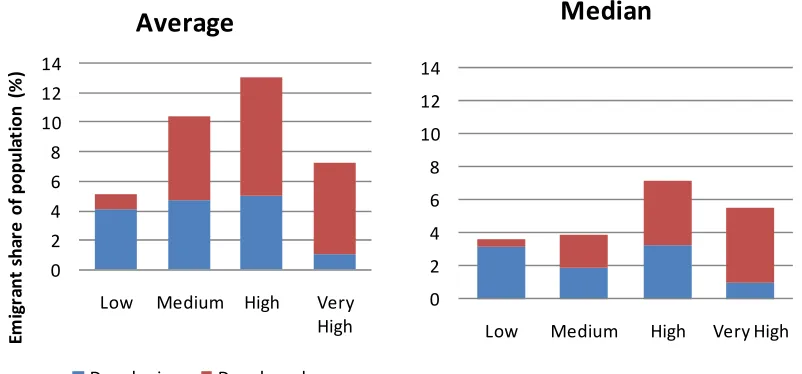
emigration rates, at least until a certain development level is achieved.3 For example, the
median emigration rate in countries with low levels of human development is 3.66, in
contrast to that in countries with high levels of human development—7.18.4 Because of these
patterns, some historians and migration scholars have hypothesized the existence of an
inverted-U relationship between development and emigration based on either cross-sectional
or time-series comparisons.5
However, simply observing that development and emigration appear to display such a
non linear-relationship leaves important questions unanswered. First of all, it is not hard to
come up with a story in which such a relationship is generated by reverse causation. Further,
even if the relationship reflects causation from development to migration, one must wonder
what it is about the process of development that impacts individuals’ propensity to leave or
stay. It may be rising income, but it may also be other socioeconomic and demographic
changes brought about by, contributing to, or simply associated with rising income.
Ultimately, people don’t just take a decision to migrate. They decide to migrate to another
country, which is why one should try to take into account the characteristics of receiving
and sending countries, as well as of the idiosyncratic forces affecting pairs of countries in any
2 For instance, in 2005, European Commission’s President José Manuel Barroso stated, on the occasion of the EC
approval of the European Union Strategy for Africa that “the problem of immigration, the dramatic consequences of which we are witnessing, can only be addressed effectively in the long term through an ambitious and coordinated Development cooperation to fight its root causes”, and the following year Nicolas Sarkozy, then France’s Interior Minister, stated in Rabat, Morocco, that “the development of Africa is the only solution, the only answer to the challenge of immigration”.
3A country’s emigration rate in a given year is defined as its emigrant population as a share of its total native
born population (at home and abroad) in that particular year.
4We use the Human Development Report’s country groups by levels of the home development, which is
indexed by the HDI as follows: low, 0.000-0.499; medium, 0.500-0.799; high, 0.800-0.899; and very high, 0.900-1.000. See UNDP (2009), which also refers to the last group as “developed” countries. Note that high human development countries are not considered developed countries but are rather the highest HDI group among developing countries.
complete migration model (e.g., the distance between them, the existence or absence of a
common border or language, the nature and strength of their historical ties). To take a simple
example, over 11% of Mexicans are living abroad, compared to 2% of Argentines, despite the
similar levels of development shared in both countries.6 The fact that Mexico shares a
common border with the United States, while Argentina does not share a common border
with any developed country is surely part of the explanation. The impact of such effects will
not be captured in any cross-national empirical exercise that lumps together migrants that
are going to very different places. Disentangling and estimating the effects of these various
factors in driving and shaping emigration at the global level constitutes the first objective of
this paper.
Before exposing our strategy and presenting detailed results, it is important to discuss
how we can think and what we know about both chains of causation. Let us first turn to the
effect of development on the incentive and propensity to out-migrate, focusing on the
potential effect of income. Take the example of a young Turkish woman who considers
migrating to Germany but ends up accepting a job in a newly-established joint-venture, and
consider alternatively the case of a young man in Bamako who after operating a cyber-café
for a few years uses his savings to join his relatives in France. The former example is
consistent with the idea that economic development reduces the incentive for emigration by
expanding opportunities at home. The latter case illustrates the opposite view: economic
development increases individuals’ financial propensity to emigrate by alleviating liquidity
constraints on movement.
These ideas can be represented through a very simple model illustrating the
mechanisms that may generate a non-linear relationship between income and development.
An individual decides to migrate by comparing utility of income, y, at home, Uyo , and at
destination, Uyd , with the cost of migrating, c. For simplicity, we use a Cobb-Douglas
utility function of the form Uy y , 0 1 . The migrant is prevented from moving
if the cost of migration is greater than income at origin, so we must have c ≤ yo. Suppose
also that there is a randomly distributed term e U0,b , which is the net gain in income
at destination and will vary across individuals. Let b c . We also assume for simplicity that
all individuals have the same income yo at origin. It follows that an individual migrates if
Uyd e Uyo c , subject to c yo . This result yields two possible outcomes:
1) If yo is sufficiently low, then the cost of moving is too great and emigration is
zero.
2) If yo ≥ c , then the fraction of people migrating will be given by the integral
yo
yde
Uydy
yo
yde
ydy
1
1y 1|
yo
yde
1
1yd e
1−y
o1
(1)
As yo increases, the fraction of people who migrate decreases. For higher income at
origin, there must be a greater net gain of migration to incite movement. The migration
hump is represented by Eq. (1) and illustrated in Figure 1.
fyo
0 if yo c
1
1yd e1−yo1 if yo ≥ c
(2)
The preceding discussion illustrates that it is very important to consider
non-linearities in the study of the effect of income on migration. The idea that over some range of
the development process development and emigration may go hand-in-hand has been
presented by various authors in the past. Hatton and Williamson (1998, 2003) show that
many countries that are highly developed7 today (e.g., Ireland, England, Italy, Spain,
Portugal, and the Republic of Korea) experienced rising emigration rates in the past. As these
countries grew wealthier, they also became more attractive to migrants from less developed
countries and were ultimately transformed from net emigration to net immigration countries
over a few decades.
Other authors have pointed out that this non-linear relationship also characterizes the
cross-sectional data.8 In fact, around 2000, the emigration rate of Morocco, a middle income
country with per capita GDP (PPP) of roughly $4,000, was twice as high (8.1%) as Niger’s
4.0% (with a per capita GDP of less than $2,000) and Norway’s (3.9%), which has one of the
world’s highest GDP per capita (close to $50,000 in 2007). Using Human Development Index
(HDI) categories yields a similar picture (Figure 2).
Anticipating our strategy and results, we can also point to the fact that in our OLS
regressions, the coefficients on origin income and origin income squared retain their
significance even when adding other variables, and that their respective signs (positive for
the former, negative for the latter) do confirm the existence of an inverted-U relationship
between income at origin and emigration. Overall, these facts strongly suggest that economic
development and (e)migration do tend to go hand-in-hand—i.e. are positively correlated—at
least up to a certain level of development, rather than what is typically posited in policy
circles. The results of our OLS regression (1) indicate that 75% of countries in our sample are
located on the upward sloping portion of the hump.
But the model that we sketched above suggests that comparisons that are only
centered on origin countries may be missing a fundamental part of the picture. In fact,
equation (2) predicts that both income at origin and destination countries matter and that
they matter nonlinearly. This suggests that models of migration that use either (i) a
cross-sectional analysis with countries as the unit of observation and thus do not distinguish
between migration among different country-pairs, or (ii) a simple linear relationship where
migration either increases or decreases with income levels or differentials, may be severely
mis-specified. To the best of our knowledge, our paper is the first attempt to address these
two specification issues simultaneously.
A third issue that arises in the analysis of how migration evolves with development is
that we would also expect migration to have an effect on economic efficiency and income.
These effects may differ by level of development. For example, emigration may foster
economic growth among poorer countries where it can alleviate labor market pressures
while providing much-needed revenue and foreign-exchange via remittances. However, in
countries with higher levels of income and overall development (including better education
systems), high rates of emigration could result in the loss of human capital that is necessary
for the development of high-technology industries and overall further development progress.
Such a pattern would generate an inverted-U relationship between migration and income
that would nevertheless not reflect causation from income to migration.
This paper attempts to deal with the need to understand the migration-development
nexus through an analysis of bilateral migration stocks that takes nonlinearities in origin and
destination income seriously while simultaneously tackling issues of causality through the
use of convincing instruments. This is achieved by estimating a model of bilateral migration
stocks using the World Bank/Sussex Database of Bilateral Migrant Stocks9 (hereafter the
Sussex matrix) from which we extract information on bilateral migrant stocks for 127
countries. We deal with the endogeneity of income to emigration using European Settler
Mortality (ESM) rates as instruments for income to isolate its exogenous component and
potential causal effect on emigration. Our research builds on the work of Acemoglu,
Johnson, and Robinson (2001) (hereafter, AJR), who have shown that ESM rates explain
contemporary differences in development through their effect on past and present-day
institutions. Subsequently, we deal with the endogeneity of emigration by constructing the
geographically-determined fraction of bilateral migrant stocks from our gravity model of
bilateral stocks and using them as instruments to estimate the effect of migration on income
both at origin and at destination for the 127 countries in our sample.
Our key findings can be summarized as follows. First, we confirm in the model of
bilateral flows the existence of a robust non-linear inverted-U relationship between income
at origin and emigration. Thus the migration ‘hump’ pattern exists in the more demanding
empirical specification of bilateral migration stocks. Second, we show that the relationship
survives in the simplest of our instrumental variables specifications. The relation appears to
be particularly fragile to controlling for destination country income and variables capturing
the economic, historical and cultural proximity between source and destination countries.
Third, when we study the effect of migration on income we do not find a robust effect on
either origin or destination income. This supports the idea that migration is not an important
contributor nor hindrance to development and that may be best seen in terms of the
expanded opportunities that it offers individuals to carry out their life plans.10
The rest of this paper is structured as follows. Section two reviews the current state of
knowledge on international migration patterns, especially those works that have focused on
the migration-development nexus and/or used gravity models of migration. In section three,
we present our strategy and data. Our results are exposed and discussed in section four.
Section five concludes.
2.
Theoretical
and
Literature
Review
The migration-development nexus has received considerable attention in the
literature. This section focuses on two sets of studies in the field: those that have analyzed
the empirical relationship between income and development using national-level data, and
those that have used gravity models to analyze the determinants and/or effects of
migration—often understood as immigration. Our paper is at their intersection of these two
literatures.
A considerable body of work has dealt with the non-linear relationship that
characterizes the effect of development on migration. The term ‘migration hump’ seems to
have been coined by Martin (1993) when discussing the likely effects of NAFTA (North
American Free Trade Agreement) on irregular migration from Mexico to the United States.
Martin argued that NAFTA would stimulate migration in the short to medium run by
fostering labor supply and mobility—especially from rural areas—before eventually reducing
the incentives to out-migrate as the income gap narrowed with the United States. Martin and
Taylor (1996) further argued that the process of social and economic development in its
broadest sense tended to be associated with generally higher levels of mobility by helping
would-be migrants pay for the fixed costs associated with migration. Only after a longer
period of sustained growth and decreasing wage gaps between origin and destination
countries would labor migration tend to decrease. According to them, emigration would tend
to decrease steeply when the income ratio between receiving and sending countries declines
from 4 or 5 to 1. Increasing income inequality would also increase people’s incentives to
migrate abroad even if average income increases.
These authors also underlined the fact that the downward-sloping portion of the
migration hump was by no means inevitable if economic growth did not result in significant
employment opportunities, in which case it could result in a semi-permanent ‘migration
plateau’ of sustained out-migration that could last for an undetermined period of time.
Olesen (2002) introduced the notion of a migration ‘band’ to refer to the income range
associated with the highest emigration rates between two countries. Olesen (2002) posited
that bilateral migration should peak and then decrease when the income differential between
the sending and the receiving countries reaches and subsequently falls below a ratio of
between 3 and 4.5 to 1, which he terms the ‘migration turning point’. More recently, de Haas
(2007) discusses how policies of rich countries that seek to stem migration by helping foster
development are ill-founded. As the poorest are empowered through economic and human
development, they will tend to move to more developed countries to realize even greater
gains, thus increasing migration rates over the short and medium terms. Hatton and
Williamson (1994, 2002, 2003, 2004, 2005) and Massey (1988, 1990, 2003) have also pointed
to historical evidence illustrating the same key fact: at low levels of income, development
Frequently applied in the study of international trade, gravity models have also been
applied to analyze the drivers of migration and how, in turn, migration affects income. As
the name suggests, gravity models are loosely derived from Newton’s law of gravitational
force and posit that the interaction between two geographic entities, through trade or
migration, are subject to forces that are inversely proportional to the distance (or income
differential) between them and on some relevant measure of their ‘masses’, including
population, area and/or income. Gravity models also typically include other geographical
controls, such as whether the country is landlocked and distance to the equator, as well as
bilateral controls that capture ‘pair-specific’ characteristics (e.g., whether two countries share
a common border, a common language, and a colonial past). The central premise behind
these models is that these structural features are likely to determine a country’s international
trade and migration patterns.
The application of gravity models to the analysis of trade goes back to Tinbergen
(1962) and Linneman (1966). Since then, gravity models have been widely used by
researchers, including Anderson (1979), Bergstrand (1985, 1989), Deardorff (1995), Frankel
and Romer (1999), Egger (2000), and Carrillo and Li (2002). Under quite similar assumptions
on the effects of geographical and other structural factors on population movement, gravity
models have also been used to study international migration.11 The overwhelming majority
of these studies have concentrated on OECD countries and used data on flows. Lewer and
Van den Berg (2008), for instance, estimated a series of gravity equations using panel data for
16 OECD countries for the period 1991–2000. Their regressions estimated bilateral flows
between countries, controlling for their populations, the distance between them, the ratio of
their per capita incomes, the pre-existing stock of foreign-born migrants, common language,
geographical contiguity (common border) and colonial ties. Other controls were also added
11 According to Lewer and Van den Berg (2008) for instance, “Immigration, like international trade, is driven by
in different specifications, such as variables for human capital and the rule of law. Their
results confirmed that international migration is indeed subject to and driven by
‘gravitational-like’ forces.
More recently, Mayda (2008) and Ortega and Peri (2009) have estimated gravity
models of international migration to developed countries. While their objectives and
specifications differ, both papers focus on international migration flows to a subset of OECD
countries for the period 1980-1995 (Mayda, 2008) and 1980-2005 (Ortega and Peri, 2009).
The authors also use panel data drawn from the OECD’s International Migration Statistics
based on OECD’s Continuous Reporting System on Migration (SOPEMI).
Mayda’s results are broadly consistent with the main theoretical predictions of
international migration theories. According to her findings, immigration flows are positively
correlated to the destination countries’ GDP per worker. However, the effect of GDP per
worker is not found to be statistically significant. These contrasting results emphasize the
importance of so-called ‘pull factors’ in driving international migration. They also underline
the complex nature of the relationship between origin country GDP and emigration, as low
income constitutes both an incentive and an impediment to movement.
Geographic and demographic factors also appear to play a major role. Hatton and
Williamson (1998, 2003) and Mayda’s (2008) results suggest that the share of the origin
country’s population aged 15-29 has a significant positive impact on outmigration (as a share
of the population). Restrictive immigration policies are found to partly offset the effect of
other push and pull factors, as, for instance, the impact of distance is greater when policies
are relaxed. These findings suggest that ‘migration quotas matter’12 and that the ‘asymmetric
effect’ between destination and home countries GDP is explained by the positive impact of
economic growth at destination on policy stance towards immigration.
A concern in most empirical studies of income is endogeneity. Mayda (2008) deals
with the endogeneity of income by relating current emigration rates to lagged values of
income and then controlling for the endogeneity of income levels with terms of trade as an
instrument. This approach would be valid only if were assumed that terms of trade have no
direct effect on migration aside from its effect through lagged income, which would not be
the case if migrants go to work in significant numbers to tradable-producing industries
which are made more profitable by a terms of trade shock.
All of these papers concentrate on the migration-development nexus in OECD
countries. To the best of our knowledge, there are no studies analyzing the effect of income
on migration using bilateral migration flows which include migration to developing
countries, and this paper is the first attempt to study the effect of development on migration
using data on migrants from and to both developing and developed countries. This is striking
because migration to non-OECD countries accounts for 51 percent of international migration
and for 65 percent of all international migration originating in non-OECD countries.13
To the best of our knowledge, only two papers have previously used bilateral
migration models to study the effect of migration on income. Both use geographical factors as
instruments, as we do. Ortega and Peri (2009) use the share of migration explained by
geography and demography as an instrument for total migration. However, their study is
limited to OECD migration data and only examines the effect of migration on destination
income—it is thus silent on the effect of migration on development as such. Felbermayr et al.
(2008) use the Sussex matrix of bilateral migration stocks (which we also use) to study the
effect of migration on income in both developed and developing countries. Similarly to us,
they use an IV technique inspired by Frankel and Romer (1999) to test the effect of
immigration on per capita income. They find that a positive and statistically significant effect
whereby their preferred specification suggests that a 10% increase in the number of migrants
leads to a 2.2% gain in per capita income. Our paper shows, however, that this effect is not
robust to adequately controlling for the endogeneity of institutions (Rodrik, et al, 2004).
3.
Empirical
Strategy
3.1.
Empirical
Model
3.1.1.OLS
In order to test for the migration ‘Hump’, we use the following empirical
specification:
lnΓij 0 1Si 2Rj 3Pijij
(3)
where Γij is the estimated stock of individuals born in country i living in country j;
S i is a vector of country-specific variables of the sending country i; R j is a vector of
country-specific variables of the receiving country j; P ij is a vector of pairwise variables
between the sending country i and receiving country j; and ij is an iid error term for
sending-receiving country pair ij. The variables that constitute S, R, and P are discussed
below with a full list and sources in Table A1.
3.1.2.Twostage least squares
To control for the endogeneity of income we use ESM rates and its square. As AJR
(2001) demonstrates, ESM rates are correlated with past and present day institutions and thus
with present-day development.14 As a result, they are exogenous to present development and
serve as an excellent candidate for an instrument. In order to use ESM as a valid instrument
for income, the one condition that we would have to accept is that they do not have an
independent effect on migration over and above that which they have on income. This
assumption may be questionable in the simplest specifications in which we do not control for
current institutions, as in such a case ESM may be correlated with the disturbance term.
However, once we control for institutions as well as a host of other country-specific
variables—and verify that the instrument maintains explanatory power in the first stage
14 In contrast to AJR (2001), in order to maintain both developed and developing countries in our sample, we set
regressions (see Table 2)—the hypothesis of a direct effect of ESM on current migration
appears much less tenable. In an alternative specification, we also include former colonial
status in the list of instruments. Again, excludability of this instrument may be questioned
but is less likely a problem in our most demanding specifications which also include
colony-colonizer pair dummies in the explanatory variables of the second stage regression.
3.2.
The
‘Horserace':
income
and
migration
Following a framework similar to that established by Rodrik, Subramanian, and
Trebbi (2004), we explore whether or not migration plays as prominent a role in a
cross-sectional analysis of income as other factors, namely institutions, trade, and geography.
3.2.1.OLS
Using OLS, we estimate the following empirical specification:
lnyi 0 1Insti 2Tradei 3Geoi 4Migi i
(4)
where i is the country index; y measures income; Inst, Trade, and Geo measure the
quality of institutions, the prevalence of trade, and geographical characteristics, respectively.
Mig represents alternatively immigration or emigration ratios (that is, the ratio of migrants
and destination or origin population), which we estimate separately. As above, i is an iid
error term.
3.2.2.Twostage least squares
In Eq. (4), we deal with the likely endogeneity of institutions, trade, and migration
using instrumental variables. In keeping with the Rodrik, et al (2004) approach, we use ESM
rates as an instrument for institutions and the Frankel-Romer measure of openness for trade.
For both immigration and emigration, we use the migration ratios explained by geographical
variables, which we know to be exogenous. More precisely, we use the predicted values of
lnΓij 0 1Distij2Borderij 3AbsLati 4Landi 5Landj ij
(5)
where Dist is the distance between origin country i and destination country j; Border
is a dummy variable that equals 1 if i and j share a common border and 0 otherwise; AbsLat is
the absolute latitude of origin country i; and Land is a dummy equal to 1 if the respective
country is landlocked and 0 otherwise. The predicted values, Γ̂ij , are then summed
separately for each origin and destination country,
∑
j1
k−1
Γ̂ij Γ̂i and
∑
i1
k−1
Γ̂ij Γ̂j,
(6)
where k 181 , the total number of countries in our sample.
Thus, Γ̂i and Γ̂j represent the geography-predicted components of immigrant and
emigrant stocks, respectively. For a single country, i , which has both an immigrant and
emigrant stock, we write Γ̂iI and Γ̂iE , using obvious notation. Dividing those by
population, we derive exogenous instruments for immigration and emigration ratios.
Estimating the endogenous variables on all of the exogenous instruments, we have the
following first-stage regressions:
Insti o 1ESMi 2ImGi 3EmGi 4FRi Inst,i
Tradei o 1FRi 2ESMi 3ImGeoi 4EmGeoi Trade,i
Imi o 1ImGeoi 2EmGeoi 3ESMi 4FRi Im,i
Emi o 1EmGeoi 2ImGeoi 3ESMi 4FRi Em,i
(7)
where ESM are European settler mortality rates; FR is the Frankel-Romer index;
ImGeo Γ̂I/Pop
and EmGeo Γ̂E/Pop
the exogenous migration rates calculated above;
3.3.
Testing
for
the
migration
‘Hump’
A key feature of our main model is that we estimate stocks—rather than flows—of
foreign-born migrants. This characteristic is a direct consequence of the paper’s goal of
extending the analysis to the whole world rather than restricting it to a small subset of rich
countries. As was previously underlined, the majority of recent papers on the subject use the
only existing reliable data on flows of international migrants to OECD countries. In contrast,
we use the only comprehensive global database—the World Bank/Sussex Bilateral Matrix—
which provides estimates for stocks in or around the year 2000. The inclusion of controls,
such as GDP per capita, life expectancy and educational attainment, reflect the
widely-viewed notion that absolute and relative levels of income and human development affect
migration patterns. Their effects, however, are complex. As discussed earlier, the propensity
to emigrate from a low-income country could increase with its level of income and/or
development, at least up to a certain point. However, it is also possible that the relationship
between the level of development and the propensity to attract migrants may be non-linear.
When the poorest are able to migrate, they may only be able to move to other very poor
countries since the barriers of moderately poor and rich countries are higher. However, once
they have sufficiently high income to overcome these barriers, they may move to the
wealthiest countries, essentially bypassing the middle income countries. As Klugman and
Pereira (2009) show, many developing countries also have high barriers to migration. Once
migrants have sufficient income to gain entrance to middle income countries, they may have
the means to gain entrance to the wealthiest countries as well. All else equal, migrants would
then tend to move to where income gains are greatest.
3.4.
Data
and
controls
We investigate how geographic, demographic, cultural, political and economic factors
affect the level and composition of the stock of international migrants living in a specific
country and groups of countries. The dependent variable is the log of the bilateral stock or
of the current knowledge and literature on potential drivers of international migration
(Yang, 2008; Massey, 1990; and Hatton and Williamson, 2002), as well as on the underlying
assumptions of gravity models.
3.4.1. Controls
Geography
Greater distance between two countries is expected to decrease the propensity of
people to move between them, as costs to move tend to increase with distance. We also
include dummy variables for countries that share a border and for landlocked countries.
Bordering countries often share a unique relationship and tend to be closely linked
politically, economically, and culturally. Migrants to or from landlocked countries also face
unique constraints since they are unable to travel by water, a common way for people to
travel cheaply over long distances.
Demography, Culture and Living Standards
Demographic factors can also influence migration patterns (Hatton and Williamson,
1998, 2003). Differences in population density and age structure between countries are likely
to have a significant impact on bilateral flows. For instance, countries with high fractions of
non-working age populations may require more workers from abroad to counteract
increasing dependency ratios, and pressure to out-migrate may be greater in countries with a
high proportion of young adults.
Countries that share a common language also tend to share other historical and
cultural ties. These commonalities can help facilitate a migrant’s integration into the host
society and labor market. Thus, countries where a potential migrant can already speak the
local language become much more attractive destinations. After controlling for income, one
could expect health and education to act as ‘pull’ factors. On the other hand, low health and
education levels imply low levels of human capital among natives at destination, which may
Political stability and governance
Environments characterized by poor governance or political instability may induce
people to move to countries where conditions are better. Politically driven migration
scenarios may vary from families that flee violent conflict as refugees to those who seek
countries where property rights are more secure or basic political freedoms are guaranteed.
On the contrary, there are reasons we may also find that higher democracy leads to lower
immigration as voters may be more likely than elites to resist immigration, particularly in
labor-scarce countries. Moreover, barriers to immigration are more likely to be effective if
the country has better institutions to enforce them.15
Economy and Trade
Particular characteristics of a nation’s economy may make it a more or less likely to be
either a net sending or receiving country. Export controls attempt to estimate whether
international migration is a substitute or a complement to trade. The contribution of the
service sector to the national economy could be a pull factor, as countries with large service
sectors may demand foreign labor. On the other hand, sectors such as services that do not
compete internationally may have more organized labor movements and be better able to
resist increased immigration.
Measurement Issues
Data on migration flows is also susceptible to more problems of measurement than
stock data. While any cross-country comparison of migration data suffers from differing
definitions of who is a migrant (some countries use place of birth while others use
nationality), flow data also tends to omit both emigrants and irregular migrants. Stock data
typically includes all migrants irrespective of their legal status, while OECD flows data only
accounts for legal immigrants. As Ortega and Peri (2009) describe, flow data often poorly
15 In principle, this could be accounted for by controlling for immigration policies, as we do. However, our
measures outflows since people who are leaving a country are less likely (or less likely to be
required) to report exiting a country.
4.
Results
4.1.
The
effect
of
development
on
migration
Let us first discuss how development affects emigration. Recall that historical and
contemporary data tend to show quite consistently that there exists a non-linear, inverted-U
shaped relationship between development at origin and emigration.
4.1.1.OLS
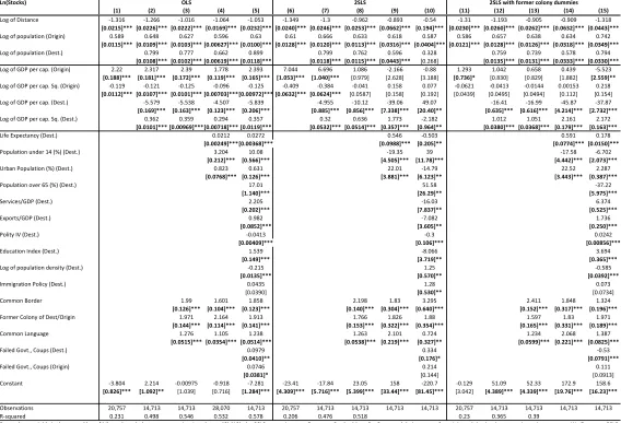
Our OLS results confirm the existence of this relationship when origin income is
allowed to pick up such non-linearity. The relationship appears to be robust as it continues to
hold even after controlling for the effect of various geographic, demographic, historical, and
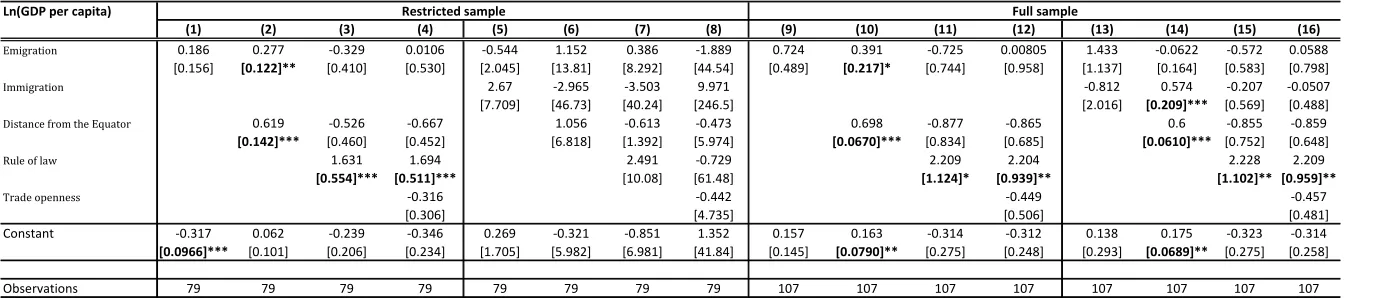
policy variables. As shown in Table 1, the coefficients on origin income and origin income
squared remain highly significant throughout regressions (1) to (5) as we progressively
control for additional explanatory variables, and their respective signs confirm the
inverted-U shape. Furthermore, their magnitude does not appear to be greatly affected by the
inclusion of these other controls.
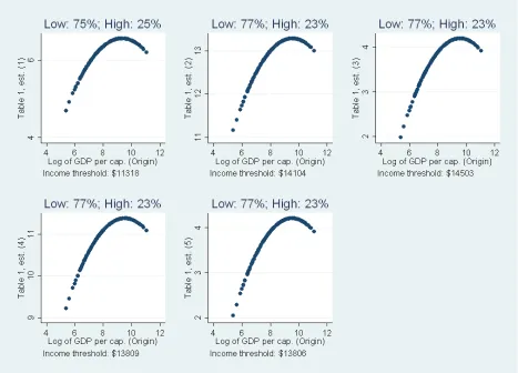
Figure 3 plots the emigration levels for varying income levels as predicted by the
coefficients yielded by regressions (1)-(5). Countries with lower income fall on the upward
sloping portion of the curve, while those with higher income fall on its downward sloping
portion. We estimate that for roughly three-quarters of countries in our sample, higher
income is associated with higher emigration. We also estimate that emigration reaches a
maximum at an income level of around $14,500, which is higher than the GDP per capita of
countries like Libya and Malaysia in 2007.
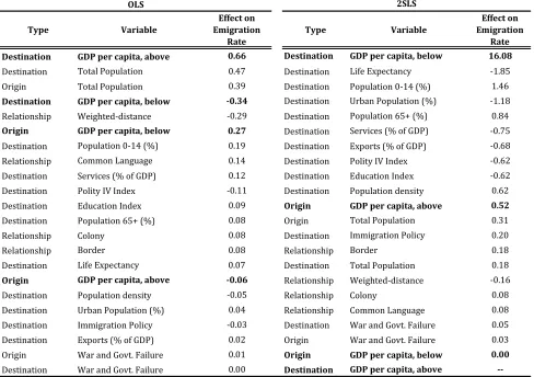
To give a sense of the intensity of the relationship, in Table 3 we calculate the
standardized coefficients corresponding to Table 1. The standardized coefficients provide an
deviation change that a particular independent variable has on migrant stocks.16
Standardized coefficients were calculated for income separately for countries located on
either portion of the curve. The standardized coefficients for the OLS model suggest that
among the set of relatively less developed countries (i.e., those located on the upward sloping
portion of the hump) a rise in income by one standard deviation in an average sending
country is associated with a 27% increase in the number of migrants located in an average
destination country. For countries located on the downward portion of the hump, an
increase in income is associated with a 6% decrease in emigration.
This finding is interesting in itself. It suggests that if cross-sectional patterns are any
indication of future trends, then we should expect that rising income in the vast majority of
countries in the world will be associated with higher emigration in the foreseeable future,
not the opposite. At this point, however, because of potential endogeneity, we are unable to
tell whether this robust relationship between income at origin and emigration reflects a
direct causal effect of the former on the latter. As described in Sections 1 and 3, we
subsequently used ESM rates as instruments for income (and their squared terms for the
squared income terms) in our regressions in order to address endogeneity concerns.
4.1.2.Twostage least squares
First stage
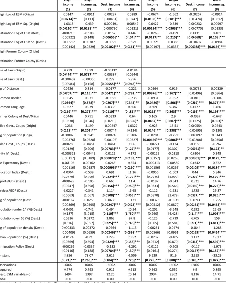
We first need to confirm that our instruments are valid. Following AJR (2001), we are
confident that ESM rates are largely exogenous—in any event today’s levels of development
and income cannot influence them. Subsequently, we need to check that they are correlated
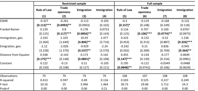
with income today. Table 2 reports the results of various variations of our first stage
regressions. These results confirm that each of our four instrumental variables is strongly
16 We calculate the standardized coefficients of income for countries above and below each threshold as follows:
sdi * [b(inci) + [ 2*b(inc2i) * meani]]
where sd is the standard deviation of income (measured as the natural log of GDP per capita) below/above the threshold, b(inc) and b(inc2) are the OLS coefficients of income and income-squared, respectively, mean is the average of income
correlated with the potentially endogenous income variable that it is used as an instrument
for. Importantly, the statistical significance of the correlation is not subject to the inclusion
or exclusion of institutional controls. In other words, our instruments affect income through
other channels and mechanisms rather than present institutions. This is critical because, as
we will see, the origin and destination ‘Rule of law’ variables drop out of our preferred IV
specification, where we have retained only significant explanatory variables not present in
the baseline specification. The data therefore tell us that present institutions do not have a
separate effect on migration over and above that of current (instrumented) income. Finally,
we are confident that we control for a sufficiently large set of variables that may impact
emigration, so that the condition that our instruments be uncorrelated with the disturbance
term is also likely met.
Second stage regressions
The results of our 2SLS regressions are reported in panel 2 of Table 1.17 Regressions
(6) and (7) show that the inverted-U relationship survives the use of instruments for income.
In these regressions with limited controls, the coefficients on the linear and quadratic origin
income terms remain highly significant, and their respective signs continue to be consistent
with an inverted-U shape. Our calculations yield that the ‘emigration-maximizing’ level of
income according to this model and specification is around $6,000, which implies that
roughly 40% of countries in our sample would fall on the downward-sloping portion of the
hump.
These initial results suggest the existence of a non-linear causal effect of income on
emigration when controlling for destination income, population and distance alone.
However, as more controls are added, the relationship loses statistical significance and
eventually turns into a (statistically insignificant) largely upward sloping relationship.
17 We first ran a 2SLS regression including all controls in our data set. We then ran the same regression
dropping the controls that were insignificant in the first and not included in our baseline model,
As we observe, the inclusion of three variables capture exogenous characteristics of
the country-pair that account for the loss of significance of the effect of origin income. These
variables are common border, common language, and former colonial relationship. The
significance of these variables suggests that the apparent non-linear effect of income on
migration is capturing the fact that middle income countries are also ‘near’ developed
countries. These countries will therefore tend to have high emigration rates—because of
their proximity to developed countries—and simultaneously be relatively developed, at least
in comparison to other developing countries. In contrast, we also observe that the
coefficients on destination income and destination income squared retain their significance
with the inclusion of these additional controls in the fully-specified regression (10). This
suggests that for most countries rising income leads to higher immigration levels. This latter
result is consistent with the notion that as a country’s income rises, it becomes more
attractive for migrants from other countries. And while the coefficients of destination
income in (10) appear to suggest that there exists an inverted U-shaped relationship between
destination income and migration, all of the countries in our sample fall below the income
threshold on the upward-sloping part of the curve in the full specification. This pattern
suggests that while there may be a decrease in the returns of destination income to
immigration, the relationship is positive for all countries.
Other factors associated with higher levels of development are also positively
correlated with higher immigration levels and can be seen as acting as ‘pull factors’. For
example, the negative coefficient on the share of population above 65 suggests that a lower
share of working-age population tends to be associated with higher immigration levels. Our
results also show that immigration policies matter: places where policy makers are more
receptive to higher levels of immigration tend to be more popular destinations. Looking at
the standardized coefficients for our preferred 2SLS estimation in Table 3, we note that the
ten variables that have the largest impact on the size of bilateral stocks pertain to the country
In general, we find that destination country variables matter a great deal, but we
caution that the interpretation of many of these additional variables can vary with
adjustments in the specification and the selection of instruments. In order to show that this is
the case, the third panel of Table 1 reruns the same regressions with an additional set of
variables in the instrument set, namely a set of colony dummies. The argument in favor of
these instruments is that former colonial status is likely to be related to development today
and is clearly exogenous. Excludability is more questionable, although it is to a great extent
attenuated by the fact that colony-colonizer dummies are included in the set of explanatory
variables. What is important to note is that in this alternative specification the signs of
several of the explanatory variables change—such as life expectancy, education, and
democracy. However, what is important for our key coefficients of interest is that the
inverted-U relationship between income and migration disappears once controls are
introduced (in fact, the specification with the most controls actually delivers a negative
linear relationship).
4.2.
The
effect
of
migration
on
development
Now that we have explored how income levels have both push and pull effects, we
examine the effect migration itself has on income. As Rodrik, et al (2004) show, when
comparing three widely analyzed channels of growth—trade, institutions, and geography—
while using instruments to control for endogeneity, the positive effect of institutions appears
to dominate all other channels. Using a similar approach, we add migration into the
equation—using geographical instruments—and observe whether migration plays a similar
role in development. Felbermayr, Hiller, and Sala (2008) have performed a similar analysis
finding a positive significant effect of migration on income, but include additional variables
for market size and financial openness, whose exogeneity is questionable and fail to
instrument for institutions.
In contrast to Felbermayr, et al (2008), we closely follow the approach pioneered by
only on exogenous variables. This is achieved either by using variables which are naturally
exogenous (e.g., geography) or by instrumenting for endogenous variables. In such a strategy,
omitted variable bias is not a concern: as we are certain of the exogeneity of the explanatory
variables, any correlation between them and an omitted variable would reflect causality from
the former to the latter. However, introducing endogenous controls in the regressions, as
Felbermayr, et al (2008) do, can seriously bias the coefficient estimates on the exogenous
variables.18
In Table 4, we show the results of our estimations of GDP per capita on immigration,
geography, institutions, and trade openness.19 Immigration is instrumented by the predicted
values of a regression of the log of immigrant stocks on several exogenous geographical
variables: log of bilateral distance, a dummy variable for a shared border, absolute latitude of
the origin country, and dummy variables for origin and destination landlocked countries.
Rule of law measures institutional quality and is instrumented by ESM rates. Trade openness
is instrumented by the geography-based Frankel-Romer openness index. In the restricted
sample, we use only countries with available ESM rates data.20 In the full sample, we set ESM
rates equal to zero for former colonial powers and ex-Soviet countries. We focus our analysis
on the full 2SLS estimations, (13)-(14).21
While immigration enters positive and highly significant in the simpler
specifications—as found by Felbermayr, et al (2008)—it becomes insignificant whenever
institutions are accounted for. In the full 2SLS estimation, the effect of immigration vanishes
with the addition of rule of law. Moreover, in the fully specified model, (16), its magnitude is
18 See Wooldridge (2002).
19 In order to compare the magnitude of each variable’s effect, we standardize all regressors by subtracting the
mean and dividing by the standard deviation.
20 This sample is the same as that used by Rodrik, et al (2004).
21 In addition to increasing the total number of observations, the power of the instruments appears stronger in
very small, indicating that even if there is an effect, its impact is negligible compared to the
other channels. In
Table 5 we find that emigration has an even less pronounced effect, while institutions
continue to dominate, further confirming the results of Rodrik, et al (2004). In Table 5 we
also include both immigration and emigration and find that their effect remains small and
insignificant while institutions persist. Our results confirm the finding of Rodrik, et al (2004)
that institutions trump other sources of growth after endogeneity is properly accounted for.
In sum, we fail to find any conclusive evidence suggesting that migration has a
substantial effect on development, much less one that rivals that of institutions.
5.
Conclusions
Studies of the relationship between migration and development have traditionally had
to deal with a set of distinct issues that hampered meaningful analysis. One is the need to
properly account for the existence of a non-linear relationship between income and
development, as suggested by many theoretical specifications. The second one is the need to
take into account that migration decisions are affected by variables in both destination and
origin countries and thus cannot be studied by the use of country aggregates that do not
distinguish by both source and destination of migrants. A third issue is the need to study a
process in which reasonable hypotheses about both directions of causation between
development and income have been postulated.
This paper has addressed these three issues by presenting empirical estimates of a
gravity model of bilateral migration that properly accounts for non-linearities and tackles
causality issues through an instrumental variables approach. In contrast to previous
contributions in this literature, which were limited to migration to OECD countries, we have
estimated the model using a matrix of bilateral migration stocks for 127 countries (Migration
DRC, 2007), allowing us to properly take into account migration to developing countries
This exercise delivers a set of interesting results. First, the inverted-U relationship (or
‘migration hump’) between income at origin and income survives the more demanding
bilateral stocks specification even after adding a large set of controls capturing conditions at
home and destination as well as pair-specific variables. Second, although the relationship also
survives in the basic IV estimation, it loses significance as we add more variables in the IV
specification. Our two alternative IV specifications (which differ in the instrument list)
deliver a similar message: the inverted-U does not survive the addition of controls for
variables that capture the characteristics of destination economies or exogenous
characteristics of the destination-origin pair.
It is best to illustrate these results with an example. Consider the cases of Morocco,
Turkey and Mexico, all three countries with moderate levels of development. The high
emigration rates of these three countries (9.0, 4.2 and 8.1 percent, respectively, as opposed to
a world average of 3 percent) appear to confirm the migration ‘hump’ hypothesis whereby
emigration rates increase and then decline with development. But these three countries also
border highly developed regions (the United States and Europe). Furthermore, their high
levels of development (in comparison to other countries in their respective regions) may
arguably be caused by their proximity to developed countries. We can only distinguish
between the effect of proximity and the effect of development if we can convincingly have
exogenous sources of variation in development, which we obtain through our IV techniques.
Once we do that, we find that proximity sweeps out the effect of development in both of our
specifications. So while it is true that countries with middle levels of development have
greater emigration rates, this appears to be caused by their proximity (geographical and
cultural) to developed countries rather than the development process.
This paper has also studied the effect that migration has on both destination and
origin country income by using geographically-induced differences across nations in
immigration and emigration as sources of exogenous variations. In the spirit of Rodrik et al.
(2004), we run a ‘horse-race’ between migration, institutions, trade and geography. While
trumped by that of institutions, so that our preferred specification fails to find any significant
effect of either immigration or emigration on income. This evidence supports the hypothesis
that migration is best viewed from the standpoint of the scope that it offers to enhance
individual opportunities rather than through its effect on aggregate economic performance.
References
Acemoglu, Johnson, and Robinson. 2001. The colonial origins of comparative development.
American Economic Review. 91: 1369-1401.
Anderson, J.E. 1979. A Theoretical Foundation for the Gravity Equation. American
Economic Review. 69: 106-116.
Bergstrand, J. 1985. The Gravity Equation in International Trade: Some Microeconomic
Foundations and Empirical Evidence. Review of Economics and Statistics 67(3):
474-481.
---. 1989. The Generalized Gravity Equation, Monopolistic Competition, and the
Factor-Proportions Theory in International Trade. Review of Economics and Statistics
71(1):143-153.
Borjas, G. 1999. Heaven’s Door. Princeton: Princeton University Press.
Carillo, C. and C. Li. 2002. Trade Blocks and the Gravity Model: Evidence from Latin
American Countries. Economics Discussion Papers No. 542. University of Essex,
Department of Economics.
Chen, L. C. and J. I. Boufford (2005), “Fatal flows—Doctors on the move”, New England
Journal of Medicine 353 (17): 1850-1852.
de Haas, H. (2007) “Turning the tide? Why development will not stop
migration”. Development and Change 38(5).
---. 2008. The Myth of Invasion: The Inconvenient Realities of African Migration to
Europe. Third World Quarterly. 29(7): 1305
Deardorff, A. 1995. Determinants of Bilateral Trade: Does Gravity Work in a Neoclassical
World? National Bureau of Economic Research Working Paper No. 5377: Cambridge,
Egger, P. 2000. A Note on the Proper Econometric Specification of the Gravity Equation.
Economics Letters. Volume 66(1): 25-31.
Felbermayr, G., S. Hiller, and D. Sala. 2008. Does Immigration Boost Per Capita Income?
Working Papers 08-23. University of Aarhus, Department of Economics.
Frankel, J. and D. Romer. 1999. Does trade cause growth? American Economic Review.
89:379-399.
Hatton, T. and J. Williamson. 1994. What Drove the Mass Migrations from Europe in the
Late Nineteenth Century? Population and Development Review. 20(3) 533–59.
---. 1998. The Age of Mass Migration: Causes and Economic Impact. New York: Oxford
University Press.
---. 2002. What Fundamentals Drive World Migration? National Bureau of Economic
Research Working Paper No. W9159. Cambridge, MA.
---. 2003. Demographic and Economic Pressure on Emigration Out of Africa. Scandinavian
Journal of Economics 105(3) 465–86.
---. 2004. Refugees, Asylum Seekers and Policy in Europe. Cambridge MA National Bureau
of Economic Research Working Paper No.10680.
---. 2005. Where Are All the Africans? Global Migrations: Two Centuries of Policy and
Performance. MIT Press: Cambridge.
Klugman, J. and I. M. Pereira. 2009. “Assessment of National Migration Policies”. Human
Development Research Paper No. 48. New York: United Nations Development
Programme, Human Development Report Office.
Lewer, J. and Van den Berg, H. 2008. A Gravity Model of Immigration. Economics Letters.
Volume 99(1): 164-167.
Linneman, H. 1966. An Econometric Study of International Trade Flows, Amsterdam:
Martin, P. 1993. Trade and Migration: NAFTA and Agriculture. Washington D.C.: Institute
for International Economics.
--- and J. Taylor. 1996. “The anatomy of a migration hump,” in J.E. Taylor (ed.),
Development Strategy, Employment and Migration: Insights from Models.
Paris:OECD, pp.43-62.
Massey, D.S. 1988. “International migration and economic development in comparative
perspective”. Population and Development Review. 14:383-413.
---. 1990. “Social Structure, Household Strategies, and the Cumulative Causation of
Migration”. Population Index 56(1): 3-26.
---. 4-7 June, 2003. “Patterns and Processes of International Migration in the 21st Century.”
Presented at the conference on African Migration in Comparative Perspective,
Johannesburg, South Africa.
Mayda, A. 2008. International Migration: A Panel Data Analysis of the Determinants of
Bilateral Flows. Center for Economic Policy and Research Discussion Paper No. 6289.
Migration DRC (Development Research Centre). 2007. “Global Migrant Origin Database
(Version 4)”. Development Research Centre on Migration, Globalisation and Poverty.
University of Sussex.
Mills, E. J., W. A. Schabas, J. Volmink, R. Walker, N. Ford, E. Katabira, A. Anema, M. Joffres,
P. Cahn, and J. Montaner (2008). “Should active recruitment of health professionals
from sub-Saharan Africa be viewed as a crime?” The Lancet 371 (9613): 685-688.
OECD (Organisation for Economic Co-operation and Development). 2009. OECD Database
on Immigrants in OECD Countries. http://stats.oecd.org/index.aspx?lang=en. Accessed
August 2009.
Olesen, H. 2002. Migration, Return and Development: An Institutional Perspective.
Ortega, F. and G. Peri. 2009. The Causes and Effects of International Labor Mobility:
Evidence from OECD Countries 1980-2005. Human Development Research Paper No.
6. New York: United Nations Development Programme, Human Development Report
Office.
Rodrik, D., A. Subramanian, and F. Trebbi. 2004. Institutions Rule: The Primacy of
Institutions Over Geography and Integration in Economic Development. Journal of
Economic Growth. Volume 9(2): 131-165.
Tinbergen, J. 1962. Shaping the World Economy: Suggestions for an International Economic
Policy. The Twentieth Century Fund: New York.
UN (United Nations). 2008. “World Population Policies 2007”. New York: UN Departement
of Social and Economic Affairs.
UNCTAD (United Nations Conference on Trade and Development). 2007. The Least
Developed Countries Report 2007: Knowledge, Technological Learning, and
Innovation for Development. New York: United Nations.
UNDP (United Nations Development Programme). 2009. Human Development Report 2009:
Overcoming Barriers. New York: Palgrave Macmillan.
Wooldridge, J.M. 2002. Econometric Analysis of Cross Section and Panel Data. Cambridge:
MIT Press.
World Bank. 2006. Global Economic Prospects: Economic Implications of Remittances and
Migration 2006. Washington DC: World Bank.
---. 2007. “Global Migrant Origin Database.”
http://www.migrationdrc.org/research/typesofmigration/global_migrant_origin_datab
ase.html. Accessed August 2009.
---. 2009. World Development Report 2009: Reshaping Economic Geography. Washington
Yang, D. 2008. "International Migration, Remittances and Household Investment: Evidence
from Philippine Migrants' Exchange Rate Shocks," Economic Journal, Royal
Economic Society 118(528): 591-630.
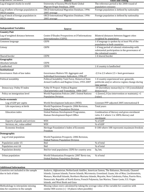
Data
sources
We merge data on the estimated stocks of international migrants with information on
geographic, cultural, institutional, socio-economic, and demographic factors from origin and
destination countries. Our source for data on international migrants is the University of
Sussex/World Bank Global Migrant Origin Database. This consists of a 226x226 bilateral
matrix of origin and destination stocks derived from the 2000 round of national population
censuses. We use the fourth version, which combines place of birth and citizenship reporting
mechanisms to create the first single, complete matrix of worldwide international migrant
stocks. The fourth version is also the most up-to-date version available at this time (March
2007). Given the extensive list of independent variables required by our model (see below),
we restrict the matrix size to 127x127 due to the limited data available for many of the
smaller countries (i.e., New Caledonia and San Marino) as well as for irregular or politically
complex countries (i.e., Afghanistan, North Korea, and West Bank and Gaza). Overall, this
reduces the estimated sample size from 175 million to 166 million worldwide migrants (or
95% of the estimated total).
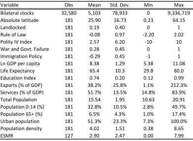
Data sources and summary statistics for all of the regressors used in the empirical
model are documented in Appendices 1 and 2. Geographic and cultural information,
including weighted distance between countries, common language, colonial ties, shared
border, absolute latitude and whether a country is landlocked, comes from the Centre
d’études prospectives et d’informations internationales (CEPII). Institutional measures come
from a variety of sources: governance is based on the Rule of Law Index from Governance
Matters VII, political instability is based on the Political Instability Task Force, democracy is
based on the Polity IV Index and immigration policy is based on the World Population
Policies from the United Nations. Regarding socio-economic data, GDP per capita and
exports and services as a percentage of GDP are derived from the World Development
Indicators; life expectancy and the education index are derived from the United Nations; and
Finally, all demographic variables, including total population, the age structure of the
population, population density and urban population, are derived from the United Nations
Population Division. All independent variables correspond to the average value for the