http://dx.doi.org/10.4236//jamp.2016.44083
How to cite this paper: Martinez, O.S., Cruz, D.M., Chavarín, J.U. and Bustos, E.S. (2016) Recurrence Quantification Analysis of Rough Surfaces Applied to Optical and Speckle Profiles. Journal of Applied Mathematics and Physics, 4, 720-732. http://dx.doi.org/10.4236//jamp.2016.44083
Recurrence Quantification Analysis of
Rough Surfaces Applied to Optical and
Speckle Profiles
Oscar Sarmiento Martinez1, Darwin Mayorga Cruz2*, Jorge Uruchurtu Chavarín2,
Estela Sarmiento Bustos3
1Technological Institute of Zacatepec-ITZ, Metal Mechanical Department, Electromechanical Engineering,
Calzada Tecnológico, Zacatepec, Mexico
2Center for Research in Engineering and Applied Sciences-CIICAp, Av. Universidad, Chamilpa, Cuernavaca,
Mexico
3Emiliano Zapata Technological University-UTEZ, Industrial Mechanics Area, Av. Universidad Tecnológica, Col.
Palo Escrito, Emiliano Zapata, Mexico
Received 16 March 2016; accepted 24 April 2016; published 27 April 2016
Copyright © 2016 by authors and Scientific Research Publishing Inc.
This work is licensed under the Creative Commons Attribution International License (CC BY).
http://creativecommons.org/licenses/by/4.0/
Abstract
In this paper, Recurrence Quantification Analysis (RQA) is set as a practical nonlinear data tool to
establish and compare surface roughness (Ra) through percentage parameters of a dynamical
sys-tem: Recurrence (%REC), Determinism (%DET) and Laminarity (%LAM). Variations in surface roughness of different machining procedures from a typical metallic casting comparator are ob-tained from scattering intensity of a laser beam and expressed as changes in the statistics of speckle patterns and profiles optical properties. The application of the analysis (RQA) by Recur-rence Plots (RPs), allowed to distinguish between machining procedures, highlighting features that other methods are unable to detect.
Keywords
RQA, Recurrence Plots, Roughness, Optical Data Processing, Speckle Patterns
1. Introduction
conditions [1]. On the other hand, the “machinability” term may be generalize as “the ease or difficulty with
which a material can be machined” [2]. However, characterizations of surfaces generated with machining
processes are usually base on conventional methods as heigth registering by means of mechanical devices, where accuracy, scanning time and surface damage are consider as disadvantages to use it for surface roughness and shape information extraction. As machining processes, like other physical systems, may evolve in multiple spatial and temporal scales ruled by complex dynamics, mathematical transformation-based techniques as
frequency and/or wavelets analysis have been developed to apply them on surface roughness characterization [3]
[4]. Nevertheless, such techniques use conventional parameters as average roughness (Ra) and mean-square
roughness (Rrms) to detect changes related to profile amplitudes, and for this reason an alternative technique
which does not depend on such parameters is also necessary.
Chaos theory may be considered for surface height fluctuations treatment, as it takes phenomena, which in spite of their apparent random nature, they are governed by deterministic laws which produce complex results as
they are mutually combined. Among different chaotic signals analysis methodologies, Echmann et al. proposed
the so called Recursive Plots (RPs) method [5]. This kind of signal graphic analysis reveals characteristics where
heterogeneities and complicated contributions of the system are highlighted, impossible to detect by means of
other different methodologies. In order to quantify the complex structure observed on RPs, Webber et al.
proposed the Recurrence Quantification Analysis (RQA), which is based on quantification of the diagonal line
structures of RPs[6]. Later, Norbert Marwan succesfully added quantifications based on vertical line structures
[7]. On the other hand, Kolmogorov Entropy (K) is a quantitative measure of the rate of information loss of a
system dynamics, where information loss in chaotic systems arises from the exponential divergence of very close trajectories. For periodic system its value is zero; for pure random system its value is positive infinity, making it impossible to predict the state of the system, and for the case of chaotic system, its value is finite and
positive [8]. More recently, Pincus [9] introduced the Approximate Entropy (ApEn) to quantify the regularity
and complexity of time series; its computing is based on the probability that patterns on a time series continue to
be similar to the next ones on incremental comparisons; ApEn has been applied as a tool to detect changes on
regularities [10], characterization of rotatory machines [11] and identification of dynamical unstabilities on
machinary processes [12][13].
The development of several non-contactive methods for surface roughness quantification is a well known
topic, being optical techniques the most widely used to measure surface features [14]-[18]. In such a context, the
speckle laser technique has been applied on different engineering and science areas, as for example to obtain roughness control parameters on metals and polymers using digital speckle patterns and optical profiles,
respectively [14]-[23]. It may be thought that combined utilization of these non-contactive techniques with those
based on non-linear data analysis as RPs, would complicate the problem making it into something intangible;
nevertheless, recent studies stablished RQA as a valid technique to compare machinability on steels as same as
metalic wearing on milling and vibration on turning processes, based on speckle images [2][24][25]. The aim
of our present work is to introduce RQA and Kolmogorov Entropy methods as practical analysis tools to
com-pare surface roughness (Ra) from different machining processes with known surface roughness. Analysis data,
obtained from a scattered laser beam, reveal changes on statistical properties of optical speckle patterns as re-lated to corresponding mechanical changes.
2. Experimental Setup and Analysis Tools
2.1. Optical Profiles and Speckle PatternsA λ = 533 nm, 50 mW output power green DPSS laser was used as the light source. A 40× microscope objective
combined with a f = 50 mm biconvex lens were used to expand and collimate the laser beam. An Alfa a 200
CCD camera with a 3872 × 2592 pixels resolution and 6.095 × 7.253 mm pixel size was used for capturing and
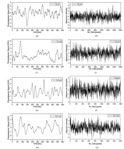
recording of speckle patterns. A roughness comparator (Microfinish, Figure 1) was used as the sample to be
il-luminated by the laser to obtain optical profiles and speckle patterns corresponding to the comparator sections characterized by different roughness ranges: 0.1 - 0.2 µm (lapped), 0.4 - 0.8 µm (rectified) and 1.6 - 12.7 µm (profiled). The green laser beam was directed to a point in the central part of each section to be analyzed on the
comparator (Figure 2(a)), where a mechanical translational system allowed the longitudinal displacement
through the sections in order to obtain the corresponding optical point scanning. The generated scattered light at
Figure 1. Microfinish surface roughness comparator.
Figure 2. Experimental setup: λ = 533 nm, Plaser = 50 mW, θ= 45˚, flens = 50 mm. (a) Point-to-point optical profiles
obtaining, (b) Surface speckle patterns obtaining.
collected by means of a biconvex lens (f = 200 mm) and directed to a power photodetector coupled to a data
ac-quisition unit, which was also coupled to a PC in order to record it for latter analysis. For speckle optical
patterns obtaining (Figure 2(b)), the green laser beam was amplified to a ∼10 mm diameter with a 40X
micro-scope objective combined with a f = 50 mm biconvex lens. A ∼78.53 mm2 area of the comparator was
illumi-nated with the laser beam considering that its corresponding reflected speckle pattern, recorded with a CCD Alfa a 200 camera, contains the variations and irregularities existing on this surface area.
An application software was used for digital data processing of each recorded speckle pattern. Intensity
pro-files (1 × 1616 pixel vectors) corresponding to ∼78.53 mm2 illuminated cross-section were obtained; the
result-ing vector represents the image average intensity profile which also contains information about surface varia-tions and irregularities of the considered surface area.
2.2. RPs and RQA
The point-to-point and surface speckle optical profiles were used to perform a qualitative analysis of the
consi-dered surface section of the comparator by means of RPs; for a quantitative analysis the RQA technique were
also used. The Visual Recurrence Analysis application software (VRA Ver. 4.9) was used for RPs building [26];
here an one-dimensional time series is expanded to a high-dimensional space where underlying system
dynam-ics is generated inside an artificial phase-space called embedding space[27], and where trajectories in the
re-build space are topologically equivalent to the original space [28]. For such a reason, determination of time-
delay (τ) is necessary to perform a correct rebuild of the process dynamics, same as a proper embedding
dimen-sion (m). The mutual information function is used for optimal delay time value determining and also for
phase-space rebuilding [29]; if optimal time-delay value is too short, the coordinates used for rebuild could be
Moreover, if optimal time-delay is too long, coordinates may be random with respect to each other. For
embed-ding dimension value selection (m), the false nearest neighbor method is used [30]. The m value determines the
number of components of the states-system rebuild vector where for noiseless time series, using embedding di-mension high values causes no problems. Oh the other hand, for time series containing noise, this is amplified
and the quality of prediction is deteriorated, so it is necessary to fix a proper m value, in such a way that the
sys-tem dynamics is optimally resolved.
In this work, the Commandline Recurrence Plots application software was used for complex structures
quan-tification [31], where only these RQA following parameters were considered: Recurrence Rate (%REC),
Deter-minism (%DET) and Laminarity (%LAM). Recurrence Rate is the percentage of recurrence points in the
phase-space, excluding main diagonal points:
, 2 , 1
1
%REC= N
∑
i jN=Ri j (1).Implicit periodic processes are characterized by higher %REC values. Determinism is the percentage of
re-currence points forming parallel segments on the main diagonal, which length reaches or exceeds minimum
length threshold; %DET allows to tell between dispersed recurrence points and those points organized in
di-agonal patterns, and contains information about duration of a stable interaction as longer is an interaction, as
higher is the %DET value:
( )
min , , % N l l N i j i j lP l DET R = =∑
∑
(2)where l is diagonal line length parallel to the identity line; P(l) is the frequency distribution of diagonal lines and
Rij is the recurrence of a state. Laminarity is the percentage of recurrence points included in linear segments
vertical to the diagonal; %LAM measures chaotic transitions and is related to the quantity of laminar phases in
the system (intermittence):
( )
( )
min 1 % N v v N v vP v LAM vP v = = =∑
∑
(3).2.3. Kolmogorov Entropy (K) and Approximate Entropy (ApEn)
The Kolmogorov Entropy is a measure of information loss index (o gain) along an attractor of certain data set.
Numerically speaking, K may be estimated as the Rényi Entropy, being the Information Theory of Shannon
En-tropy a particular case. On the other hand, the product of the Shannon EnEn-tropy and the Boltzmann constant is the
Thermodynamic Entropy [8]. The Kolmogorov Entropy is defined as follows [8][32]:
( )
( )1 2 1 2
0 , , , , , ,
1 1
lim lim lim ln
1 N N
m r q
q r t N i i i i i i
K X p
N t q →∞ ∆→ →∞
= −
∆ −
∑
(4)where {X = xi} is the random variable and x x t i ti =
(
= ∆)
; 1 2, , ,Nq i i i
p is the joint probability than x (t = ∆t)
tra-jectory is in the i1, x (t = 2∆t) in i2, and x (t = N∆t) in iN. Here, application software RRCHAOS [33] have been
applied for the maximum-likelihood estimation of Kolmogorov Entropy (KML), proposed by Schouten [34];
KML is usually expressed in bits/seconds, where a finite positive value (0 < KML < ∞) means that underlying
time series/data is chaotic, a value equal to zero (KML = 0) represents an ordered system (regular, cyclic or
con-stant), and an infinite value (KML →∞) infers that the system is an stochastic one (random) [8].
The Approximate Entropy (ApEn) quantifies the regularity and complexity in real time series, where time
se-ries with higher ApEn values may present considerable irregularity fluctuations (more complex), while lower
ApEn values would indicate more regular time series (less complex). Given its simplicity, ApEn has been
ap-plied in many fields of science and engineering including psychology, geophysics and financial systems. A
de-tailed description of the method may be found on specialized literature [8]-[11]. The Approximate Entropy
es-timated for a finite value N is defined by:
(
, ,)
1 m(
, ,)
(m1)(
, ,)
.s
ApEn m m m
T
ε τ = ∅ ε τ − ∅ + ε τ
For calculation of ApEna Matlab code implementation by Danny Kaplan was used here [35][36].
3. Results and Discussion
3.1. Data Series and Computed Parameters
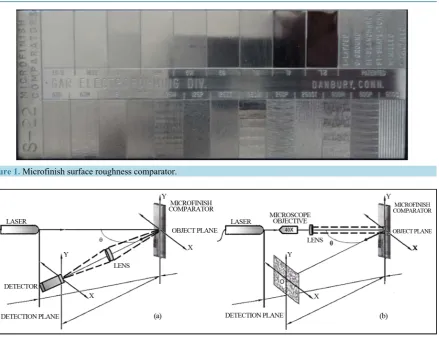
In Figure 3, data series of optical profiles and speckle patterns are shown, corresponding to different
conven-tional machineries which surface roughness vary between Ra= 0.2 - 12.7 µm.
For qualitative (RPs) and quantitative (RQA) optical and speckle profiles analysis, a mutual information
func-tion analysis was performed to obtain the optimal time-delay value (τ) and consequently, by using the false
neighbor method, it was used to obtain the embedding dimension value (m) where maximum dimension value
was set on 10 and then, from obtained τ and computed m, RPs were generated with VRA software [26]. The
cor-responding RQA analysis was performed using Commandline Recurrence Plots software [31] considering τ and
m values; the average phase-space diameter was also computed to obtain the optimal Threshold Radius (ε) [36]
[37]. A set of the parameters described above is shown in Table 1.
3.2. Qualitative Analysis
The analysis consisted in generating RPs from the optical and speckle patterns of different machining processes
for different surface roughness degrees. In Figure 4, corresponding RPs generated without threshold value ε are
displayed.
0 200 400 600 800 1000 1200 1400 1600 -2 -1 0 1 2 3 M ax im um Int ens ity
No. Data [pixels]
0.2 µm
(a) (b)
0 50 100 150 200 250 300 350 400 450 500 -3 -2 -1 0 1 2 3 Phot odet ec tor S ignal [V DC ] time [sec]
0.4 µm
0 200 400 600 800 1000 1200 1400 1600
-4 -3 -2 -1 0 1 2 3 4 M ax im um Int ens ity
No. Data [pixels]
0.4 µm
(c) (d)
0 50 100 150 200 250 300 350 400 450 500 -2 -1 0 1 2 3 Phot odet ec tor s ignal [V DC ] time [sec]
0.8 µm
0 200 400 600 800 1000 1200 1400 1600
-4 -3 -2 -1 0 1 2 3 4 M ax im um Int ens ity
No. Data [pixels]
0.8 µm
(e) (f)
0 50 100 150 200 250 300 350 400 450 500 -3 -2 -1 0 1 2
3 0.2 µm
0 50 100 150 200 250 300 350 400 450 500 -4 -3 -2 -1 0 1 2 3 Phot odet ec tor S igna [ VD C ] time [sec]
1.6 µm
0 200 400 600 800 1000 1200 1400 1600 -4 -3 -2 -1 0 1 2 3 4 5 M ax im um Int ens ity
No. Data [pixels]
1.6 µm
(g) (h)
0 50 100 150 200 250 300 350 400 450 500 -2 -1 0 1 2 3 4 Phot odet ec tor S ignal [V DC ] time [sec]
3.2 µm
0 200 400 600 800 1000 1200 1400 1600 -3 -2 -1 0 1 2 3 4 M ax im um Int ens ity
No. Data [pixels]
3.2 µm
(i) (j)
0 50 100 150 200 250 300 350 400 450 500 -2 -1 0 1 2 3 Phot odet ec tor S ignal [V DC ] time [sec]
6.4 µm
0 200 400 600 800 1000 1200 1400 1600 -3 -2 -1 0 1 2 3 M áx im os de I nt ens idad
No. Datos [pixels]
6.4µm
(k) (l)
0 50 100 150 200 250 300 350 400 450 500 -3 -2 -1 0 1 2 3 Phot odet ec tor S ignal [V D C ] time [sec]
12.7 µm
0 200 400 600 800 1000 1200 1400 1600 -3 -2 -1 0 1 2 3 4 M ax im um Int ens ity
No. Data [pixels]
12.7 µm
(m) (n)
Figure 3. Optical and speckle profiles, (a) (b): Lapped, Ra= 0.2 µm. (c) (d): Rectified, Ra= 0.4 µm. (e) (f): Rectified, Ra= 0.8 µm. (g) (h): Profiled, Ra = 1.6 µm. (i) (j): Profiled, Ra = 3.2 µm. (k) (l): Profiled, Ra = 6.4 µm. (m) (n): Profiled, Ra = 12.7 µm.
The information about the dynamics of a time series/data is usually obtained from the density of points and
line structures in a RPs[25]; a recursive homogeneous plot without a structure typically indicates an
autonom-ous or stationary process such as white noise, unlike oscillating systems which present periodic recurrent or di-agonally orientated structures (diagonal lines or discernible patterns). The presence of vertical or horizontal lines indicates a presence of intermittence or laminarity, whereas sudden changes on the process or the dynamics as
[image:6.595.85.522.80.603.2](a) (b)
(c) (d)
(g) (h)
(i) (j)
(m) (n)
Figure 4. RPs obtained from optical and speckle patterns: (a) (b): Lapping, Ra = 0.2 µm. (c) (d): Rectified, Ra = 0.4 µm. (e) (f): Rectified, Ra = 0.8 µm. (g) (h): Profiled, Ra = 1.6 µm. (i) (j): Profiled, Ra = 3.2 µm. (k) (l): Profiled, Ra = 6.4 µm. (m) (n): Profiled, Ra = 12.7 µm.
Table 1. Parameters computed for RPs and RQA analysis.
Process Surface Speckle pattern resolution: 1616 × 1080 pixels Ra
[µm]
Optical profiles Speckle profiles
τ m ε τ m ε
Lapped 0.2 29 10 3.54 5 4 2.04
Rectified
0.4 23 10 3.54 4 4 2.76
0.8 29 5 2.55 5 5 3.03
Profiled
1.6 26 10 3.45 3 3 2.44
3.2 38 4 2.16 5 5 3.13
6.4 30 7 2.46 3 3 2.43
[image:9.595.83.539.373.725.2]As it can be observed on Fig. 4, surface roughness Ra offers an initial visual inspection for identification of
changes on dynamics of the structure, reflected on RPs textures which are defined as small scale patterns and
revealed by the color and/or texture type (generated by the machining process) in the RP. The optical profiles
(Figure 3(a), Figure 3(c), Figure 3(e), Figure 3(g), Figure 3(i), Figure 3(k), Figure 3(m)) and their
corres-ponding RPs (Figure 4(a), Figure 4(c), Figure 4(e), Figure 4(g), Figure 4(i), Figure 4(k), Figure 4(m))
present certain discernible patterns or diagonally oriented structures as surface roughness increases; this agrees
with surface texture of each process shown on Table 1, which might implies that sharp cutting forces produced
during machining process generate very regular signals, and therefore a better machinability. On the other hand,
speckle profiles (Figure 3(b), Figure 3(d), Figure 3(f), Figure 3(h), Figure 3(j), Figure 3(l), Figure 3(n)) only
present vertical and horizontal lines as roughness degree increases, which indicate no presence of oscillations
with some periodicity (i.e. no correlation among them), and also implying a stochastic behavior. This last may
be related to the effect of surface roughness on the speckle pattern formation (Table 1), where this generates a
random intensity distribution, as the result of multiple interference of light scattered from each irregularity on the rough surface.
3.3. Quantitative Analysis
Although RPs offer an initial visual comparison of surface roughness, it is necessary to evaluate it in a
quantita-tive way. In order to perform Recurrence Quantification Analysis (RQA), the m, τ, and εparameters (indicated in
Table 1) are necessary, as also to consider the Euclidean distance as a parameter to determine the distance
be-tween new vectors; in our case a minimum diagonal of 2 was considered. In Figure 5(a) the Recurrence Rate
(%REC) was calculated for optical and speckle profiles as a function of surface roughness Ra; the
age %REC for the profiles was 47.69% y 60.23%, respectively, which implies that analyzed surface textures
were generated by processes with certain degree of periodicity.
0.1 1 10
0 10 20 30 40 50 60 70 80 90 100
%
R
ec
ur
renc
e
Ra [µm]
Optical profiles Speckle profiles
(a)
0.1 1 10
80.0 82.5 85.0 87.5 90.0 92.5 95.0 97.5 100.0
%
D
et
er
m
ini
sm
Ra [µm]
Optical profiles
Speckle profiles
(b)
0.1 1 10
90 91 92 93 94 95 96 97 98 99 100
%
Lam
inar
ity
Ra [µm] Optical profiles
Speckle profiles
(c)
The calculated Determinism (%DET) is shown in Figure 5(b), where high %DET values can be adverted for
different Ra degrees. The average %DET was 99.756% for optical profiles and 91.534% for speckle ones; this is
reflected on surface texture nature of machining processes (see Table 1 images) as %DET reaches higher values
when machining produces signals with more stable (regular) correlation and interaction degrees, due to cutting forces presented in the process. Unlike the above, if cutting forces during machining process were unstable
(ir-regular), it may generate signals with low %DET values, and therefore, a low machinability.
In Figure 5(c), the calculated Laminarity (%LAM) is presented; as %LAM may be defined as an alternation of
states or phases in dynamical systems, in our particular case this could be interpreted as the alternation of regular
(stable) and irregular (unstable) surface textures, due to cutting forces. The average value %LAM for optical and
[image:11.595.186.442.480.692.2]speckle profiles was 99.856% and 95.006%, respectively.
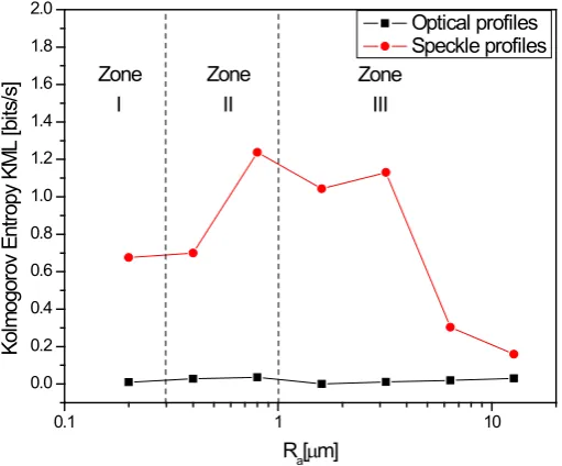
Figure 6 represents the maximum likelihood Kolmogorov Entropy (KML) calculated from optical and speckle
series. For the optical ones, KML exhibit a lower rate of information creation for every lapping, rectified and
profiled cases, where an average value KML = 0.02 bits/seg was obtained; this value is characteristic for regular
oscillating (certain periodicity degree) and therefore less complex series, which is reflected on the optical
pro-files shown in Figure 3. For the case of speckle profiles, a KML = 0.676 bits/seg (Ra = 0.2 µm) correspond to
the zone I (lapping process); at zones II (rectified process) and III (profiled process), increments with maxima
values at KML = 1.237 bits/seg (Ra = 0.8 µm), KML = 1.043 bits/seg (Ra = 1.6 µm) and KML = 1.13 bits/seg (Ra
= 3.2 µm) were obtained. Such increments may be associated with a high sensitivity to external conditions or
perturbations as the alternation of regular and irregular texture surfaces, for example, presented on speckle pat-tern intensities.
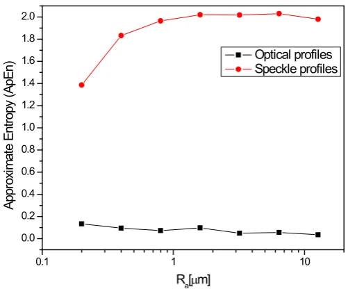
Regarding Approximate Entropy (ApEn) calculation shown in Figure 7, for optical profiles the obtained
ApEn = 0.07717 low average value evidences the presence of regular oscillations, while for speckle profiles the
calculated ApEn = 1.89, higher than obtained for optical profiles, may be associated to different irregularities
between the processes as surface roughness increases, which reflected on the speckle pattern intensities. An
ad-vantage of ApEn with respect to KML is its computational effectiveness as same as its algorithm, which may
produce acceptable results from certain relatively small number of observations.
4. Conclusion
The RQA, KML and ApEn analysis methods can be suggested as practical comparison tools for the surface
roughness (Ra) on different reliefs. From the presented results and considerations, one might conclude that such
techniques are very sensitive to changes on mechaning conditions and can be thoroughly employed to establish
0.1 1 10
0.0 0.2 0.4 0.6 0.8 1.0 1.2 1.4 1.6 1.8 2.0
Zone Zone
Kol
m
ogor
ov
E
nt
ropy
K
M
L [
bi
ts
/s
]
Ra[µm]
Optical profiles Speckle profiles
I II III
Zone
Figure 6. Maximum likelihood Kolmogorov Entropy for optical and
0.1 1 10 0.0
0.2 0.4 0.6 0.8 1.0 1.2 1.4 1.6 1.8 2.0
Appr
ox
im
at
e E
nt
ropy
(A
pE
n)
Ra[µm]
[image:12.595.188.439.82.290.2]Optical profiles Speckle profiles
Figure 7. ApEn analysis of optical and speckle profiles as a function of surface roughness Ra.
and compare the machinability of different types of metallic materials. A combined application of optical methods together with those based on nonlinear data analysis is here outlined.
References
[1] Guerrero, F.E.L., Flores, R.C. and Acosta, M.D. (2003) Caracterización de Superficies Maquinadas por Medio de Parámetros de Rugosidad. Ingenierías, 6, 62-68.
[2] Ravish, U.K.S., Alva, A., Gangadharan, K.V. and Desai, V. (2011) Recurrence Quantification Analysis to Compare the Machinability of Steels. ARPN Journal of Engineering and Applied Sciences, 6, 8-13.
[3] Litak, G., Syta, A. and Rusinek, R. (2011) Dynamical Changes during Composite Milling: Recurrence and Multiscale Entropy Analysis. International Journal of Advanced Manufacturing Technology, 56, 445-453.
http://dx.doi.org/10.1007/s00170-011-3195-8
[4] Bethencourt, M., Botana, F.J., Calvino, J.J., Marcos, M. and Rodríguez-Chacón, M.A. (1998) Aplicación del Análisis de Fourier al Estudio de Perfiles de Rugosidad de Muestras Erosionadas. Revista de Metalurgia, 34, 7-11.
http://dx.doi.org/10.3989/revmetalm.1998.v34.iExtra.698
[5] Eckmann, J.P., Kamphorst, S.O. and Ruelle, D. (1987) Recurrence Plots of Dynamical Systems. Europhysics Letters, 4, 973-977. http://dx.doi.org/10.1209/0295-5075/4/9/004
[6] Webber, C.L. and Zbilut, J.P. (1994) Dynamical Assessment of Physiological Systems and States Using Recurrence Plot Strategies. Journal of Applied Physiology, 76, 965-973.
[7] Marwan, N. (2003) Encounters with Neighbours—Current Developments of Concepts Based on Recurrence Plots and Their Applications. PhD Thesis, Institute for Physics, University of Potsdam, Potsdam.
[8] Liu, M. and Hu, Z. (2014) Nonlinear Analysis and Prediction of Time Series in Multiphase Reactors. In: Liu, M., Ed., Springer Briefs in Applied Sciences and Technology, Springer International Publishing, New York, 1-44.
http://dx.doi.org/10.1007/978-3-319-04193-3
[9] Pincus, S.M. (1991) Approximate Entropy as a Measure of System Complexity. Proceedings of the National Academy of Sciences of the United States of America, 88, 2297-2301. http://dx.doi.org/10.1073/pnas.88.6.2297
[10] Restrepo, J.N., Shlotthauer, G. and Torres, M.E. (2014) Maximum Approximate Entropy and Threshold: A New Ap-proach for Regularity Changes Detection. Physica A, 409, 97-109.
[11] Yan, R., Liu, Y. and Gao, R.X. (2012) Permutation Entropy: A Nonlinear Statistical Measure for Status Characteriza-tion of Rotary Machines. Mechanical Systems and Signal Processing, 29, 474-484.
http://dx.doi.org/10.1016/j.ymssp.2011.11.022
[13] Pérez-Canales, D., Vela-Martinez, L., Jáuregui-Correa, J.C. and Álvarez-Ramírez, J. (2012) Analysis of Entropy Ran-domness Index for Machining Chatter Detection. International Journal of Machine Tools & Manufacture, 62, 39-45.
http://dx.doi.org/10.1016/j.ijmachtools.2012.06.007
[14] Sherwood, K.F. and Crookall, J.R. (1967-1968) Surface Finish Assessment by an Electrical Capacitance Technique. Proceedings of the Institution of Mechanical Engineers, 182, 344-349.
[15] Blessing, G.V. and Eitzen, E.D. (1998) Surface Roughness Sensed by Ultrasound. Surface Topography, 1, 143-158. [16] Sosa Correa, W.O., Sierra, M., Parra Vargas, C.A. and Salcedo, L.A. (2006) Análisis de Rugosidad por Microscopía de
Fuerza Atómica (AFM) y Software SPIP Aplicado a Superficies Vítreas. Revista Colombiana de Física, 38, 826-829. [17] Peña Sierra, R., Romero-Paredes, R.G. and Águila Rodríguez, G. (2001) Estudio de la Morfología Superficial e Índice
de Refracción en Películas Nanométricas de Silicio Poroso. Superficies y Vacío, 13, 92-96.
[18] Sherrington, I. and Smith, E.H. (1988) Modern Measurement Techniques in Surface Metrology: Part I. Stylus Instru-ments, Electron Microscopy and Non-Optical Comparators. Wear, 125, 271-288.
http://dx.doi.org/10.1016/0043-1648(88)90118-4
[19] Sherrington, I. and Smith, E.H. (1988) Modern Measurement Techniques in Surface Metrology: Part II. Optical In-struments. Wear, 125, 289-308. http://dx.doi.org/10.1016/0043-1648(88)90119-6
[20] Sampaio, A.L., Lobao, D.C., Nunes, L.C.S., Dos Santos, P.A.M., Silva, L. and Huguenin, J.A.O. (2011) Hurst Expo-nent Determination for Digital Speckle Patterns in Roughness Control of Metallic Surfaces. Optics and Lasers in En-gineering, 49, 32-35. http://dx.doi.org/10.1016/j.optlaseng.2010.09.005
[21] Marbán, A., Sarmiento-Martínez, O., Mayorga-Cruz, D., Menchaca, C. and Uruchurtu, J. (2010) Polymer Surface Roughness Determination throughout the Hurst Analysis from Optical Signal Measurements. Journal of Materials Science and Engineering, 4, 26-31.
[22] Menchaca, C., Nava, J.C., Valdéz, S., Sarmiento-Martínez, O. and Uruchurtu, J. (2010) Gamma-Irradiated Nylon Roughness as Function of Dose and Time by the Hurst and Fractal Dimension Analysis. Journal of Materials Science and Engineering, 4, 50-58.
[23] Elias, J. and Rajesh, V.G. (2010) Detection of Chatter in Turning Using Recurrence Plot Analysis of Input Current, Vibration of Tool and Speckle Image of Machined Surface. International Journal of Production Technology and Management (IJPTM), 1, 56-64.
[24] Mhalsekar, S.D., Rao, S.S. and Gangadharan K.V. (2010) Investigation on Feasibility of Recurrence Quantification Analysis for Detecting Flank Wear in Face Milling. International Journal of Engineering, Science and Technology, 2, 23-38. http://dx.doi.org/10.4314/ijest.v2i5.60098
[25] http://visual-recurrence-analysis.software.informer.com/4.9/
[26] Takens, F. (1993) Detecting Nonlinearities in Stationary Time Series. International Journal of Bifurcation and Chaos, 3, 241-256. http://dx.doi.org/10.1142/S0218127493000192
[27] Cazares Ibáñez, E.A. (2005) Estudio de sistemas caóticos y su relación con el fenómeno de corrosión por picadura en un sustrato metálico en presencia de iones cloruro y sulfato. PhD Thesis, Facultad de Química, UNAM,México, D.F. [28] Fraser, A.M. and Swinney, H.L. (1986) Independent Coordinates for Strange Attractors from Mutual Information.
Physical Review A, 33, 1134-1140. http://dx.doi.org/10.1103/PhysRevA.33.1134
[29] Kennel, M.B., Brown, R. and Abarbanel, H.D.I. (1992)Determining Embedding Dimension for Phase-Space Recon-struction Using a Geometrical ConRecon-struction. Physical Review A, 45, 3403-3411.
http://dx.doi.org/10.1103/PhysRevA.45.3403
[30] http://tocsy.pik-potsdam.de/CRPtoolbox/crp_man.pdf
[31] Grassberger, P. and Procaccia, I. (1983) Estimation of Kolmogorov Entropy from a Chaotic SIGNAL. Physical Review A, 28, 2591-2593. http://dx.doi.org/10.1103/PhysRevA.28.2591
[32] Schouten, J.C., Takens, F. and Van den Bleek, C.M. (1994) Maximum-Likelihood Estimation of the Entropy of an At-tractor. Physical Review E, 49, 126-129. http://dx.doi.org/10.1103/PhysRevE.49.126
[33] Schouten, J.C., Takens, F. and Van den Bleek, C.M. (1994) Estimation of the Dimension of a Noisy Attractor. Physical Review E, 50, 1851-1861. http://dx.doi.org/10.1103/PhysRevE.50.1851
[34] http://www.macalester.edu/~kaplan/hrv/doc/
[35] https://www.physionet.org/physiotools/ApEn/
[36] Shinkel, S. Dimigen, O. and Marwan, N. (2008) Selection of Recurrence Threshold for Signal Detection. The Euro-pean Physical Journal Special Topics, 164, 45-53. http://dx.doi.org/10.1140/epjst/e2008-00833-5
[37] Zbilut, J.P., Thomasson, N. and Webber, C.L. (2002) Recurrence Quantification Analysis as a Tool for Exploration of Nonstationary Cardiac Signals. Medical Engineering & Physics, 24, 53-60.